Quantum Computing (fall2013) Instructor:Shengyu Zhang. Lecture 10 Quantum information 2:entropy and mutual information 1.Review of classical information theory Let's first review some basic concepts in information theory. Suppose that X is a discrete random variable on the sample space X,and the probability distribution function is p(x)=Pr [X =x].Following the standard notation in information theory,we also use the capital letter X to denote the distribution,and by writing x-X,we mean to draw a sample x from the distribution X. Entropy.The entropy H(X)of a discrete random variable X is defined by H0=-∑plo8p). XEX Here we use the convention that 0log2 0=0. One intuitive explanation about this definition is that entropy measures the amount of the uncertainty of a random variable.The more entropy X has,the more uncertain it is.In particular,H(X)=0 iff X is fixed/deterministic.At the other extreme,the maximum entropy for any random variable on X is log?X,achieved by the uniform distribution.The range of the entropy is 0≤H(X)≤log2l, Another interpretation of entropy is the compression rate,which will be the subject of the next lecture A special case is binary entropy,when X takes only 2 possible values.Suppose Pr[X p,then the binary entropy is H(p)plog(1-p)ogHow does this quantity vary with p?See the following figure
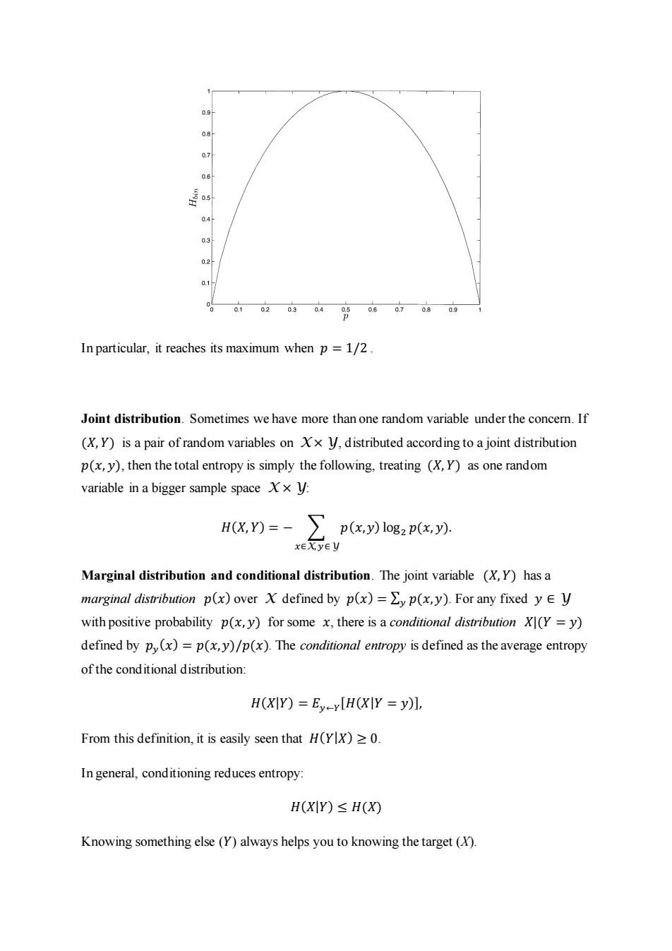
Quantum Computing (Fall 2013) Instructor: Shengyu Zhang. Lecture 10 Quantum information 2: entropy and mutual information 1. Review of classical information theory Let’s first review some basic concepts in information theory. Suppose that 𝑋 is a discrete random variable on the sample space X, and the probability distribution function is 𝑝(𝑥) = Pr [𝑋 = 𝑥]. Following the standard notation in information theory, we also use the capital letter 𝑋 to denote the distribution, and by writing 𝑥 ← 𝑋, we mean to draw a sample 𝑥 from the distribution 𝑋. Entropy. The entropy 𝐻(𝑋) of a discrete random variable 𝑋 is defined by 𝐻(𝑋) = − ∑𝑝(𝑥) log2 𝑝(𝑥) 𝑥∈X . Here we use the convention that 0log2 0 = 0. One intuitive explanation about this definition is that entropy measures the amount of the uncertainty of a random variable. The more entropy 𝑋 has, the more uncertain it is. In particular, 𝐻(𝑋) = 0 iff 𝑋 is fixed/deterministic. At the other extreme, the maximum entropy for any random variable on X is log2 |X|, achieved by the uniform distribution. The range of the entropy is 0 ≤ 𝐻(𝑋) ≤ log2 |X|, Another interpretation of entropy is the compression rate, which will be the subject of the next lecture. A special case is binary entropy, when 𝑋 takes only 2 possible values. Suppose Pr[𝑋 = 𝑥] = 𝑝, then the binary entropy is 𝐻(𝑝) = 𝑝 log 1 𝑝 + (1 − 𝑝) log 1 1−𝑝 . How does this quantity vary with 𝑝? See the following figure
07 0.6 05 04 0.3 0.1 80. In general,conditioning reduces entropy: H(XIY)≤H(XO Knowing something else(Y)always helps you to knowing the target (X)
In particular, it reaches its maximum when 𝑝 = 1/2 . Joint distribution. Sometimes we have more than one random variable under the concern. If (𝑋, 𝑌) is a pair of random variables on X × Y, distributed according to a joint distribution 𝑝(𝑥, 𝑦), then the total entropy is simply the following, treating (𝑋, 𝑌) as one random variable in a bigger sample space X × Y: 𝐻(𝑋, 𝑌) = − ∑ 𝑝(𝑥,𝑦) log2 𝑝(𝑥, 𝑦) 𝑥∈X, 𝑦∈Y . Marginal distribution and conditional distribution. The joint variable (𝑋, 𝑌) has a marginal distribution 𝑝(𝑥) over X defined by 𝑝(𝑥) = ∑ 𝑝(𝑥,𝑦) 𝑦 . For any fixed 𝑦 ∈ Y with positive probability 𝑝(𝑥, 𝑦) for some 𝑥, there is a conditional distribution 𝑋|(𝑌 = 𝑦) defined by 𝑝𝑦 (𝑥) = 𝑝(𝑥,𝑦)/𝑝(𝑥). The conditional entropy is defined as the average entropy of the conditional distribution: 𝐻(𝑋|𝑌) = 𝐸𝑦←𝑌 [𝐻(𝑋|𝑌 = 𝑦)], From this definition, it is easily seen that 𝐻(𝑌|𝑋) ≥ 0. In general, conditioning reduces entropy: 𝐻(𝑋|𝑌) ≤ 𝐻(𝑋) Knowing something else (𝑌) always helps you to knowing the target (X)
Chain rule.Another basic fact is the chain rule: H(X,Y)=H(X)+H(Y X). Think of this as the following:The uncertainty of H(X,Y)is that of one variable X,plus that of the other variable Y after knowing X. The chain rule also works with conditional entropy, H(X,Y Z)=H(X Z+H(Y X,Z), and with more variables: H(Xi,...Xnl2)=H(X12)+H(X2IX,Z)+.+H(XnlX...,Xn-1,Z) ≤H(XlZ)+H(X2lZ)+…+H(XnlZ), where the inequality is usually referred to as the subadditivity of entropy. Relative entropy.Another important concept is that of the relative entropy of two distributions p and q. H(pllq) p(x)logz p(x) q(x) XEX Relative entropy can sometimes serve as a good measure as distance of two measures.A basic property is that it is nonnegative. Fact.H(pllq)>0 with equality iff p=q. Proof.Use the faet that oin the definition ofH Mutual information.For a joint distribution (X,Y)=p(x,y),the mutual information between X and Y is I(X;Y)=D(p(x,y)Ilp(x)p(y))=H(X)-H(XIY)=H(X)+H(Y)-H(X,Y). It is a good exercise to verify the above equalities.But the second one has a clear explanation: We mentioned earlier that conditioning always reduces the entropy.How much does it reduce? Exactly the mutual information.So the mutual information is the amount of uncertainty of X minus that when Y is known.In this way,it measures how much Y contains the
Chain rule. Another basic fact is the chain rule: 𝐻(𝑋, 𝑌) = 𝐻(𝑋) + 𝐻(𝑌|𝑋). Think of this as the following: The uncertainty of 𝐻(𝑋, 𝑌) is that of one variable 𝑋, plus that of the other variable 𝑌 after knowing 𝑋. The chain rule also works with conditional entropy, 𝐻(𝑋, 𝑌|𝑍) = 𝐻(𝑋|𝑍) + 𝐻(𝑌|𝑋, 𝑍), and with more variables: 𝐻(𝑋1 , …, 𝑋𝑛 |𝑍) = 𝐻(𝑋1 |𝑍) + 𝐻(𝑋2 |𝑋1 ,𝑍) + ⋯ + 𝐻(𝑋𝑛 |𝑋1 ,… , 𝑋𝑛−1 , 𝑍) ≤ 𝐻(𝑋1 |𝑍) + 𝐻(𝑋2 |𝑍) + ⋯ + 𝐻(𝑋𝑛 |𝑍), where the inequality is usually referred to as the subadditivity of entropy. Relative entropy. Another important concept is that of the relative entropy of two distributions 𝑝 and 𝑞. 𝐻(𝑝||𝑞) = ∑𝑝(𝑥) log2 𝑝(𝑥) 𝑞(𝑥) 𝑥∈X . Relative entropy can sometimes serve as a good measure as distance of two measures. A basic property is that it is nonnegative. Fact. 𝐻(𝑝||𝑞) ≥ 0 with equality iff 𝑝 = 𝑞. Proof. Use the fact that log2 𝑥 = ln 𝑥 ln 2 ≤ 𝑥−1 ln 2 in the definition of 𝐻(𝑝||𝑞). Mutual information. For a joint distribution (𝑋, 𝑌) = 𝑝(𝑥,𝑦), the mutual information between 𝑋 and 𝑌 is 𝐼(𝑋; 𝑌) = 𝐷(𝑝(𝑥,𝑦)||𝑝(𝑥)𝑝(𝑦)) = 𝐻(𝑋) − 𝐻(𝑋|𝑌) = 𝐻(𝑋) + 𝐻(𝑌) − 𝐻(𝑋, 𝑌). It is a good exercise to verify the above equalities. But the second one has a clear explanation: We mentioned earlier that conditioning always reduces the entropy. How much does it reduce? Exactly the mutual information. So the mutual information is the amount of uncertainty of 𝑋 minus that when 𝑌 is known. In this way, it measures how much 𝑌 contains the

information of X.It is not hard to verify that it's symmetric:I(X;Y)=H(X)-H(XY)= H(Y)-H(YIX),and we've implicitly said that it's nonnegative: I(X;Y)≥0,i.e.I(X;Y)≤min{H(X),H(Y)} One can also add conditioning on this.The conditional mutual information is defined by I(X;YIZ)=E,[I(X;Y (Z=))] It is not hard to see that I(X;YIZ)≤min{H(XIZ),H(YIZ)}≤log2q and I(X;Y Z)=H(X Z)-H(X YZ). Data processing inequality.A sequence of random variables X1,X2,...form a Markov Chain,.denoted by X1→X2→…if Pr[Xn xIXn-1=xn-1]=Pr[Xn xIX1 =x1,...Xn-1=xn-1] Namely,X depends only on X1,but not the"earlier history". Fact.IfX→Y→Z,then I(X;Z≤I(X;Y). Intuitively,it says that processing data always reduces the contained information. 2.Quantum entropy We can extend the classical Shannon entropy to the quantum case.The von Newmann entropy of a quantum state p is defined by S(p)=-tr(p logp) Equivalently,if the eigenvalues of p are入=(,,入n),then S(p)=H().Note that tr(p)=1andp≥0,so入is a distribution.) Similar to the classical case,the quantum entropy is a measure of uncertainty of the quantum states
information of 𝑋. It is not hard to verify that it’s symmetric: 𝐼(𝑋; 𝑌) = 𝐻(𝑋) − 𝐻(𝑋|𝑌) = 𝐻(𝑌) − 𝐻(𝑌|𝑋), and we’ve implicitly said that it’s nonnegative: 𝐼(𝑋; 𝑌) ≥ 0, i.e. 𝐼(𝑋; 𝑌) ≤ min{𝐻(𝑋), 𝐻(𝑌)} One can also add conditioning on this. The conditional mutual information is defined by 𝐼(𝑋; 𝑌|𝑍) = 𝐸𝑧 [𝐼(𝑋; 𝑌 | (𝑍 = 𝑧))] It is not hard to see that 𝐼(𝑋; 𝑌|𝑍) ≤ min{𝐻(𝑋|𝑍), 𝐻(𝑌|𝑍)} ≤ log2 |X| and 𝐼(𝑋; 𝑌|𝑍) = 𝐻(𝑋|𝑍) − 𝐻(𝑋|𝑌𝑍). Data processing inequality. A sequence of random variables 𝑋1 , 𝑋2 , … form a Markov Chain, denoted by 𝑋1 → 𝑋2 → ⋯ if Pr[𝑋𝑛 = 𝑥|𝑋𝑛−1 = 𝑥𝑛−1 ] = Pr[𝑋𝑛 = 𝑥|𝑋1 = 𝑥1 ,… , 𝑋𝑛−1 = 𝑥𝑛−1 ] Namely, 𝑋𝑛 depends only on 𝑋𝑛−1 , but not the “earlier history”. Fact. If 𝑋 → 𝑌 → 𝑍, then 𝐼(𝑋;𝑍) ≤ 𝐼(𝑋; 𝑌). Intuitively, it says that processing data always reduces the contained information. 2. Quantum entropy We can extend the classical Shannon entropy to the quantum case. The von Newmann entropy of a quantum state 𝜌 is defined by 𝑆(𝜌) = −𝑡𝑟(𝜌 log 𝜌) Equivalently, if the eigenvalues of 𝜌 are λ = (λ1 , …, λ𝑛 ), then 𝑆(𝜌) = 𝐻(𝜆) . (Note that tr(𝜌) = 1 and ρ ≽ 0, so 𝜆 is a distribution.) Similar to the classical case, the quantum entropy is a measure of uncertainty of the quantum states
Fact.S(p)>0,with equality iff p is a pure state. Relative entropy.The quantum relative entropy is defined by S(pllo)=tr(plog p-ploga) Let's first verify that this extends the classical relative entropy.When p and o commute and they have eigenvalues {pi}and {qi,then solo)=∑P.loP--og)-∑,ls0 qi consistent with the classical case. The relative entropy can be viewed as a distance measure between states. Theorem(Klein's inequality).S(pllo)>0 with equality holding iff p=o. Another"distance"property is that taking partial trace reduces relative entropy. Fact.S(PAllOA)S(p) with equality iff PipPi=p. Conditional entropy.Suppose that a joint quantum system (A,B)is in state PaB.For convenience,we sometimes use (A,B)to denote PaB.We define the conditional entropy as S(AlB)=S(A,B)-S(B) Note that classically conditional entropy can also be defined as the average of S(Alb),but we cannot do it for quantum entropy.Actually,different than the classical case,the quantum
Fact. 𝑆(𝜌) ≥ 0, with equality iff 𝜌 is a pure state. Relative entropy. The quantum relative entropy is defined by 𝑆(𝜌||𝜎) = tr(𝜌log 𝜌 − 𝜌 log 𝜎) Let’s first verify that this extends the classical relative entropy. When 𝜌 and 𝜎 commute and they have eigenvalues {𝑝𝑖 } and {𝑞𝑖 }, then 𝑆(𝜌||𝜎) = ∑(𝑝𝑖 log 𝑝𝑖 − 𝑝𝑖 log 𝑞𝑖 ) 𝑖 = ∑𝑝𝑖 log 𝑝𝑖 𝑞𝑖 𝑖 consistent with the classical case. The relative entropy can be viewed as a distance measure between states. Theorem (Klein’s inequality). 𝑆(𝜌||𝜎) ≥ 0 with equality holding iff 𝜌 = 𝜎. Another “distance” property is that taking partial trace reduces relative entropy. Fact. 𝑆(𝜌𝐴 ||𝜎𝐴 ) ≤ 𝑆(𝜌𝐴𝐵 ||𝜎𝐴𝐵). The theorem can be used to prove the following result. Fact. Projective measurements can only increase entropy. More precisely, suppose {𝑃𝑖 } is a complete set of orthogonal projectors and 𝜌 is a density operator. Then 𝑆(∑𝑖 𝑃𝑖𝜌𝑃𝑖 ) ≥ 𝑆(𝜌) with equality iff 𝑃𝑖𝜌𝑃𝑖 = 𝜌. Conditional entropy. Suppose that a joint quantum system (𝐴, 𝐵) is in state 𝜌𝐴𝐵 . For convenience, we sometimes use (𝐴, 𝐵) to denote 𝜌𝐴𝐵 . We define the conditional entropy as 𝑆(𝐴|𝐵) = 𝑆(𝐴,𝐵) − 𝑆(𝐵) Note that classically conditional entropy can also be defined as the average of 𝑆(𝐴|𝑏), but we cannot do it for quantum entropy. Actually, different than the classical case, the quantum
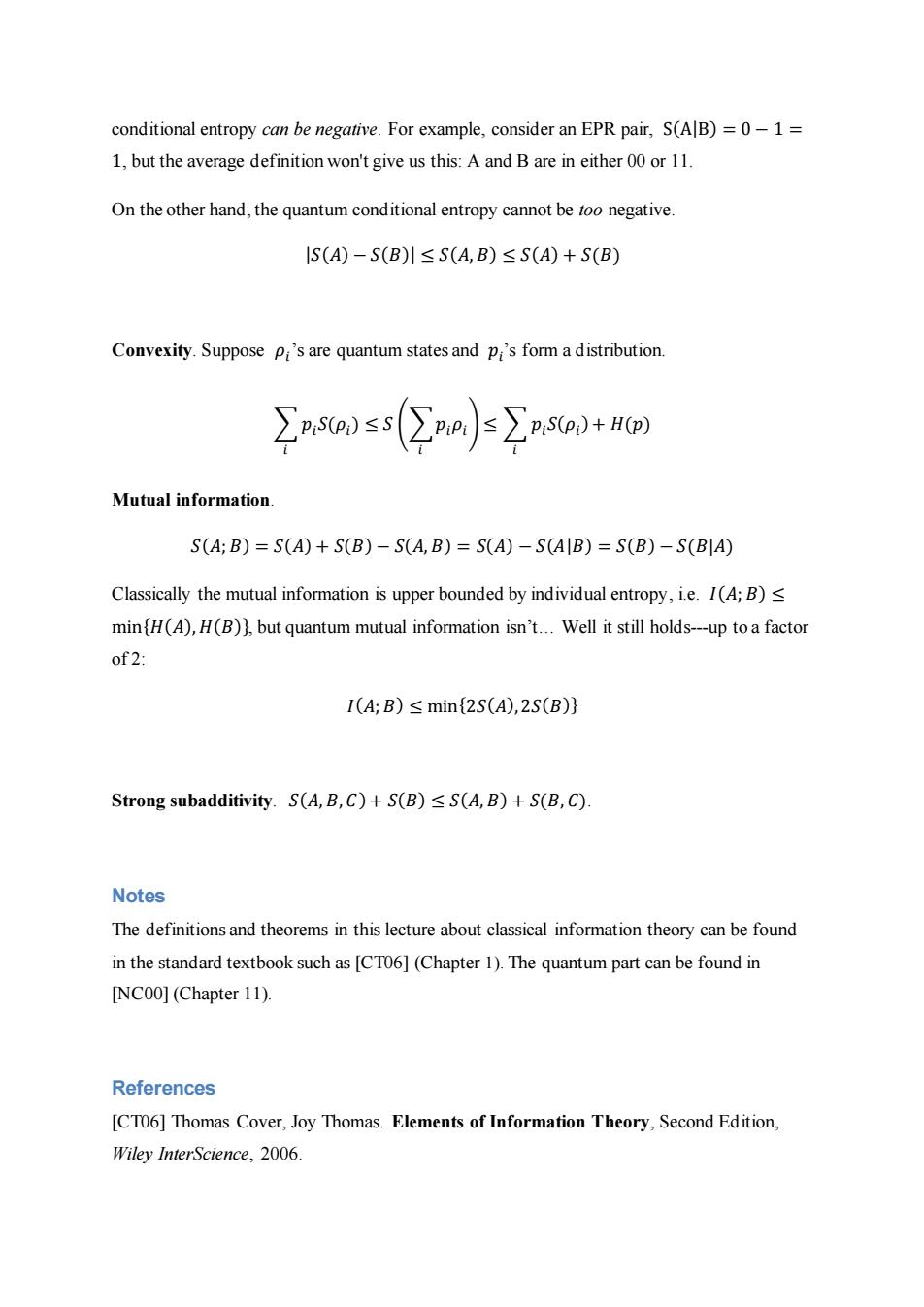
conditional entropy can be negative.For example,consider an EPR pair,S(A|B)=0-1 1,but the average definition won't give us this:A and B are in either 00 or 11. On the other hand,the quantum conditional entropy cannot be too negative. IS(A)-S(B)川≤S(A,B)≤S(A)+S(B) Convexity.Suppose Pi's are quantum states and pi's form a distribution. Mutual information. S(A;B)=S(A)+S(B)-S(A,B)=S(A)-S(AIB)=S(B)-S(BA) Classically the mutual information is upper bounded by individual entropy,i.e.I(A;B)< min(H(A),H(B)},but quantum mutual information isn't...Well it still holds---up to a factor of2: 1(A;B)<min(2S(A),2S(B)} Strong subadditivity.S(A,B,C)+S(B)<S(A,B)+S(B,C). Notes The definitions and theorems in this lecture about classical information theory can be found in the standard textbook such as [CT06](Chapter 1).The quantum part can be found in [NC0O](Chapter 11). References [CT06]Thomas Cover,Joy Thomas.Elements of Information Theory,Second Edition, Wiley InterScience,2006
conditional entropy can be negative. For example, consider an EPR pair, S(A|B) = 0 − 1 = 1, but the average definition won't give us this: A and B are in either 00 or 11. On the other hand, the quantum conditional entropy cannot be too negative. |𝑆(𝐴) − 𝑆(𝐵)| ≤ 𝑆(𝐴, 𝐵) ≤ 𝑆(𝐴) + 𝑆(𝐵) Convexity. Suppose 𝜌𝑖 ’s are quantum states and 𝑝𝑖 ’s form a distribution. ∑𝑝𝑖𝑆(𝜌𝑖 ) 𝑖 ≤ 𝑆 (∑𝑝𝑖𝜌𝑖 𝑖 ) ≤ ∑𝑝𝑖𝑆(𝜌𝑖 ) 𝑖 + 𝐻(𝑝) Mutual information. 𝑆(𝐴; 𝐵) = 𝑆(𝐴) + 𝑆(𝐵) − 𝑆(𝐴, 𝐵) = 𝑆(𝐴) − 𝑆(𝐴|𝐵) = 𝑆(𝐵) − 𝑆(𝐵|𝐴) Classically the mutual information is upper bounded by individual entropy, i.e. 𝐼(𝐴; 𝐵) ≤ min{𝐻(𝐴), 𝐻(𝐵)}, but quantum mutual information isn’t… Well it still holds---up to a factor of 2: 𝐼(𝐴; 𝐵) ≤ min{2𝑆(𝐴),2𝑆(𝐵)} Strong subadditivity. 𝑆(𝐴, 𝐵, 𝐶)+ 𝑆(𝐵) ≤ 𝑆(𝐴, 𝐵) + 𝑆(𝐵, 𝐶). Notes The definitions and theorems in this lecture about classical information theory can be found in the standard textbook such as [CT06] (Chapter 1). The quantum part can be found in [NC00] (Chapter 11). References [CT06] Thomas Cover, Joy Thomas. Elements of Information Theory, Second Edition, Wiley InterScience, 2006

[NC0O]Michael Nielsen and Isaac Chuang,Quantum Computation and Quantum Information, Cambridge University Press,2000 Exercise 1.What's the von Newmann entropy of the following quantum states? ●lp)=10) ●0)=2(I0》+1) 。。=ǖ出 2.What's the mutual information between the two parts of an EPR state?
[NC00] Michael Nielsen and Isaac Chuang, Quantum Computation and Quantum Information, Cambridge University Press, 2000. Exercise 1. What’s the von Newmann entropy of the following quantum states? ⚫ |𝜓〉 = |0〉 ⚫ |𝜓〉 = 1 √2 (|0〉 + |1〉) ⚫ 𝜌 = 1 3 [ 2 1 1 1 ]. 2. What’s the mutual information between the two parts of an EPR state?