Types of Sums of Squares With flexibility(especially unbalanced designs)and expansion in mind,this ANOVA package was implemented with general linear model(GLM)approach.There are different ways to quantify factors(categorical variables)by assigning the values of a nominal or ordinal variable,but we adopt binary coding for each factor level and all applicable interactions into dummy (indicator)variables.An ANOVA can be written as a general linear model: Y=bo+biX1+b2X2+...+bkXkte With matrix notation, Y1 ……Xk X 1…Xk en it is reduced to a simple form Y=Xb+e The design matrix for a 2-way ANOVA with factorial design 2X3 looks like Data Design Matrix A B A*B AB A1 A2 BI B2 B3 A1B1 A1B2 A1B3 A2B1 A2B2 A2B3 11 110100 1 0 0 0 0 0 12 1 10010 0 1 0 0 0 0 13 110001 0 0 1 0 0 0 21 01100 0 0 0 0 0 22 1 01010 0 0 0 0 1 0 231 01001 0 0 0 0 0 1 After removing an effect of a factor or an interaction from the above full model(deleting some columns from matrix X),we obtain the increased error due to the removal as a measure of the effect.And the ratio of this measure relative to some overall error gives an F value,revealing the significance of the effect. However,there are different approaches to keeping or removing columns of an effect, and sometimes it is a sensitive and controversial issue among statisticians
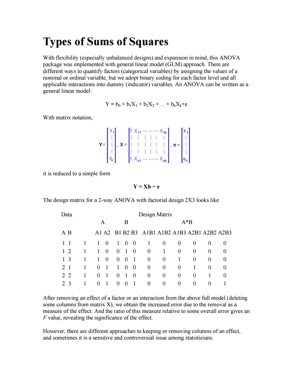
Types of Sums of Squares With flexibility (especially unbalanced designs) and expansion in mind, this ANOVA package was implemented with general linear model (GLM) approach. There are different ways to quantify factors (categorical variables) by assigning the values of a nominal or ordinal variable, but we adopt binary coding for each factor level and all applicable interactions into dummy (indicator) variables. An ANOVA can be written as a general linear model: Y = b0 + b1X1 + b2X2 + ... + bkXk+e With matrix notation, it is reduced to a simple form Y = Xb + e The design matrix for a 2-way ANOVA with factorial design 2X3 looks like Data Design Matrix A B A*B A B A1 A2 B1 B2 B3 A1B1 A1B2 A1B3 A2B1 A2B2 A2B3 1 1 1 1 0 1 0 0 1 0 0 0 0 0 1 2 1 1 0 0 1 0 0 1 0 0 0 0 1 3 1 1 0 0 0 1 0 0 1 0 0 0 2 1 1 0 1 1 0 0 0 0 0 1 0 0 2 2 1 0 1 0 1 0 0 0 0 0 1 0 2 3 1 0 1 0 0 1 0 0 0 0 0 1 After removing an effect of a factor or an interaction from the above full model (deleting some columns from matrix X), we obtain the increased error due to the removal as a measure of the effect. And the ratio of this measure relative to some overall error gives an F value, revealing the significance of the effect. However, there are different approaches to keeping or removing columns of an effect, and sometimes it is a sensitive and controversial issue among statisticians
·Type:sequential The SS for each factor is the incremental improvement in the error SS as each factor effect is added to the regression model.In other words it is the effect as the factor were considered one at a time into the model,in the order they are entered in the model selection,for example A,B,C,and D in a 4-way ANOVA.The SS can also be viewed as the reduction in residual sum of squares(SSE)obtained by adding that term to a fit that already includes the terms listed before it. Pros: (1)Nice property:balanced or not,SS for all the effects add up to the total SS,a complete decomposition of the predicted sums of squares for the whole model.This is not generally true for any other type of sums of squares. (2)Preferable when some factors(such as nesting)should be taken out before other factors.For example with unequal number of male and female,factor "gender"should precede "subject"in an unbalanced design. Cons: (1)Order matters!Hypotheses depend on the order in which effects are specified.If you fit a 2-way ANOVA with two models,one with A then B,the other with B then A,not only can the type I SS for factor A be different under the two models,but there is NO certain way to predict whether the SS will go up or down when A comes second instead of first This lack of invariance to order of entry into the model limits the usefulness of Type I sums of squares for testing hypotheses for certain designs. (2)Not appropriate for factorial designs Type II:hierarchical or partially sequential SS is the reduction in residual error due to adding the term to the model after all other terms except those that contain it,or the reduction in residual sum of squares obtained by adding that term to a model consisting of all other terms that do not contain the term in question.An interaction comes into play only when all involved factors are included in the model.For example,the SS for main effect of factor A is not adjusted for any interactions involving A:AB,AC and ABC,and sums of squares for two-way interactions control for all main effects and all other two-way interactions,and so on. Pros: (1)appropriate for model building,and natural choice for regression
• Type I: sequential The SS for each factor is the incremental improvement in the error SS as each factor effect is added to the regression model. In other words it is the effect as the factor were considered one at a time into the model, in the order they are entered in the model selection , for example A, B, C, and D in a 4-way ANOVA. The SS can also be viewed as the reduction in residual sum of squares (SSE) obtained by adding that term to a fit that already includes the terms listed before it. Pros: (1) Nice property: balanced or not, SS for all the effects add up to the total SS, a complete decomposition of the predicted sums of squares for the whole model. This is not generally true for any other type of sums of squares. (2) Preferable when some factors (such as nesting) should be taken out before other factors. For example with unequal number of male and female, factor "gender" should precede "subject" in an unbalanced design. Cons: (1) Order matters! Hypotheses depend on the order in which effects are specified. If you fit a 2-way ANOVA with two models, one with A then B, the other with B then A, not only can the type I SS for factor A be different under the two models, but there is NO certain way to predict whether the SS will go up or down when A comes second instead of first. This lack of invariance to order of entry into the model limits the usefulness of Type I sums of squares for testing hypotheses for certain designs. (2) Not appropriate for factorial designs • Type II: hierarchical or partially sequential SS is the reduction in residual error due to adding the term to the model after all other terms except those that contain it, or the reduction in residual sum of squares obtained by adding that term to a model consisting of all other terms that do not contain the term in question. An interaction comes into play only when all involved factors are included in the model. For example, the SS for main effect of factor A is not adjusted for any interactions involving A: AB, AC and ABC, and sums of squares for two-way interactions control for all main effects and all other two-way interactions, and so on. Pros: (1) appropriate for model building, and natural choice for regression
(2)most powerful when there is no interaction (3)invariant to the order in which effects are entered into the model Cons: (1)For factorial designs with unequal cell samples,Type II sums of squares test hypotheses that are complex functions of the cell ns that ordinarily are not meaningful. (2)Not appropriate for factorial designs Type III:marginal or orthogonal SS gives the sum of squares that would be obtained for each variable if it were entered last into the model.That is,the effect of each variable is evaluated after all other factors have been accounted for.Therefore the result for each term is equivalent to what is obtained with Type I analysis when the term enters the model as the last one in the ordering. Pros: Not sample size dependent:effect estimates are not a function of the frequency of observations in any group (i.e.for unbalanced data,where we have unequal numbers of observations in each group).When there are no missing cells in the design,these subpopulation means are least squares means,which are the best linear-unbiased estimates of the marginal means for the design. Cons: (1)testing main effects in the presence of interactions (2)Not appropriate for designs with missing cells:for ANOVA designs with missing cells,Type III sums of squares generally do not test hypotheses about least squares means, but instead test hypotheses that are complex functions of the patterns of missing cells in higher-order containing interactions and that are ordinarily not meaningful. Type IV:Goodnight or balanced A variation of type Ill,but spefically developed for designs with missing cells. Suppose we have a model with two factors and the terms appear in the order A,B,AB. Let R()represent the residual sum of squares for a model,so for example R(A,B,AB)is the residual sum of squares fitting the whole model,R(A)is the residual sum of squares
(2) most powerful when there is no interaction (3) invariant to the order in which effects are entered into the model Cons: (1) For factorial designs with unequal cell samples, Type II sums of squares test hypotheses that are complex functions of the cell ns that ordinarily are not meaningful. (2) Not appropriate for factorial designs • Type III: marginal or orthogonal SS gives the sum of squares that would be obtained for each variable if it were entered last into the model. That is, the effect of each variable is evaluated after all other factors have been accounted for. Therefore the result for each term is equivalent to what is obtained with Type I analysis when the term enters the model as the last one in the ordering. Pros: Not sample size dependent: effect estimates are not a function of the frequency of observations in any group (i.e. for unbalanced data, where we have unequal numbers of observations in each group). When there are no missing cells in the design, these subpopulation means are least squares means, which are the best linear-unbiased estimates of the marginal means for the design. Cons: (1) testing main effects in the presence of interactions (2) Not appropriate for designs with missing cells: for ANOVA designs with missing cells, Type III sums of squares generally do not test hypotheses about least squares means, but instead test hypotheses that are complex functions of the patterns of missing cells in higher-order containing interactions and that are ordinarily not meaningful. • Type IV: Goodnight or balanced A variation of type III, but spefically developed for designs with missing cells. ========================== Suppose we have a model with two factors and the terms appear in the order A, B, AB. Let R(·) represent the residual sum of squares for a model, so for example R(A,B,AB) is the residual sum of squares fitting the whole model, R(A) is the residual sum of squares

fitting just the main effect of A,and R(1)is the residual sum of squares fitting just the mean.The three types of sums of squares are calculated as follows: Term Type 1 SS Type 2 SS Type 3 SS A SS(A)=R(1)-R(A) SS(AB)=R(B)-R(A,B) SS(AB,AB)=R(B,AB)- R(A.B.AB) B SS(BIA)=R(A)-R(A,B) SS(BA)=R(A)-R(A,B) SS(BIA,AB)=R(A,AB) R(A,B,AB) AB SS(ABA,B)=R(A,B)- SS(ABA,B)=R(A,B)- SS(ABIA,B)=R(A,B)- R(A.B,AB) R(A,B,AB) R(A.B.AB) Their relationship: Effect Balanced Unbalanced Missing Cells A I=II=III=IV III=IV B I=II=III=IV I=II,III=IV I=II AB I=II=III=IV I=II=III=IV I=II=III=IV The type of SS only influences computations on unbalanced data.because for orthogonal designs,it does not matter which type of SS is used since they are essentially the same The nice thing about balanced designs is that orthogonality protects us from worrying about any potential interference among factors.If possible,balanced designs in group analysis are desirable by all means. In most ANOVA designs,it is assumed the independents are orthogonal(uncorrelated, independent).This corresponds to the absence of multicollinearity in regression models. If there is such lack of independence,then the ratio of the between to within variances will not follow the F distribution assumed for significance testing. Only when a design is unbalanced does the type of SS become an issue,thus the controversy over the preference on SS type.Two kinds of unbalanced designs in FMRI group analysis are: (1)Unequal number of subjects across groups (2)Missing cells:Some subjects fail to perform some tasks. Currently only two designs of the first kind are available in the package:
fitting just the main effect of A, and R(1) is the residual sum of squares fitting just the mean. The three types of sums of squares are calculated as follows: Term Type 1 SS Type 2 SS Type 3 SS A SS(A)=R(1)-R(A) SS(A|B)=R(B)-R(A,B) SS(A|B,AB)=R(B,AB)- R(A,B,AB) B SS(B|A)=R(A)-R(A,B) SS(B|A)=R(A)-R(A,B) SS(B|A,AB)=R(A,AB)- R(A,B,AB) AB SS(AB|A,B)=R(A,B)- R(A,B,AB) SS(AB|A,B)=R(A,B)- R(A,B,AB) SS(AB|A,B)=R(A,B)- R(A,B,AB) Their relationship: Effect Balanced Unbalanced Missing Cells A I=II=III=IV III=IV B I=II=III=IV I=II, III=IV I=II AB I=II=III=IV I=II=III=IV I=II=III=IV ========================== The type of SS only influences computations on unbalanced data. because for orthogonal designs, it does not matter which type of SS is used since they are essentially the same. The nice thing about balanced designs is that orthogonality protects us from worrying about any potential interference among factors. If possible, balanced designs in group analysis are desirable by all means. In most ANOVA designs, it is assumed the independents are orthogonal (uncorrelated, independent). This corresponds to the absence of multicollinearity in regression models. If there is such lack of independence, then the ratio of the between to within variances will not follow the F distribution assumed for significance testing. Only when a design is unbalanced does the type of SS become an issue, thus the controversy over the preference on SS type. Two kinds of unbalanced designs in FMRI group analysis are: (1) Unequal number of subjects across groups. (2) Missing cells: Some subjects fail to perform some tasks. Currently only two designs of the first kind are available in the package:
(1)3-way ANOVA BXC(A)(type 3):C is a random factor nested within factor A while B is a fixed factor; (2)4-way ANOVA BXCXD(A)(type 3):D is a random factor nested within factor A while B and C are two fixed factors. There is NO consensus on which type of SS should be used for unbalanced designs,but most statisticians generally recommend type III,which is the default in most software packages such as SAS,SPSS,JMP,Minitab,Stata,Statista,Systat,and Unistat while R, S-Plus,Genstat,and Mathematica use type I.However,Langsrud(2003)argues that Type II is preferable considering the power of types II and III. In the two unbalanced designs implemented so far in the Matlab package,both of them are nested/mixed designs,and it makes sense to take type I,having control factor(group) precede the primary factor(subject). Theoretical reasons aside,there is a practical consideration in this package to adopt Type I SS.All ANOVAs are built on a pure crossed (factorial)design.For example,all other 3-way ANOVA types are caluclated from the "seed"design AXBXC with all factors being fixed.In mixed design BXC(A)with A and B fixed,and C(usually subject) random and nested within A,we have SSBC(A)=SSBC+SSABC,df BC(A)=df BC+df ABC As mentioned above,this nice structure only holds with Type I SS,and would collapse with other types of SS. How much is the difference among different types of SS? Test Data Level B1 B2 B3 B4 4 35 77 Al 6 88 41 9 33 3 68 12510 A2 2 3610 2 45 23611 Three ANOVA Summary Tables
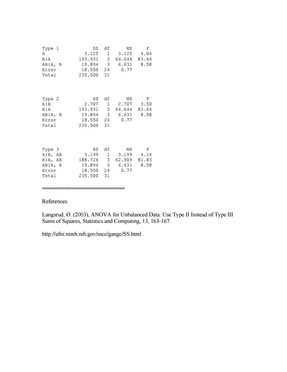
(1) 3-way ANOVA BXC(A) (type 3): C is a random factor nested within factor A while B is a fixed factor; (2) 4-way ANOVA BXCXD(A) (type 3): D is a random factor nested within factor A while B and C are two fixed factors. There is NO consensus on which type of SS should be used for unbalanced designs, but most statisticians generally recommend type III, which is the default in most software packages such as SAS, SPSS, JMP, Minitab, Stata, Statista, Systat, and Unistat while R, S-Plus, Genstat, and Mathematica use type I. However, Langsrud (2003) argues that Type II is preferable considering the power of types II and III. In the two unbalanced designs implemented so far in the Matlab package, both of them are nested/mixed designs, and it makes sense to take type I, having control factor (group) precede the primary factor (subject). Theoretical reasons aside, there is a practical consideration in this package to adopt Type I SS. All ANOVAs are built on a pure crossed (factorial) design. For example, all other 3-way ANOVA types are caluclated from the "seed" design AXBXC with all factors being fixed. In mixed design BXC(A) with A and B fixed, and C (usually subject) random and nested within A, we have SSBC(A) = SSBC + SSABC, df BC(A) = df BC + df ABC As mentioned above, this nice structure only holds with Type I SS, and would collapse with other types of SS. ======================== How much is the difference among different types of SS? Test Data Level B1 B2 B3 B4 A1 3 6 3 4 5 4 3 3 7 8 7 6 7 8 9 8 A2 1 2 2 2 2 3 4 3 5 6 5 6 10 10 9 11 Three ANOVA Summary Tables
Type 1 SS df MS d A 3.125 1 3.125 4.04 BIA 193.931 64.644 83.64 ABIA,B 19.894 3 6.631 8.58 Error 18.550 24 0.77 Total 235.500 31 Type 2 SS df MS AB 2.707 2.707 3.50 BIA 193.931 3 64.644 83.64 ⊙ ABIA, 19.894 6.631 8.58 Error 18.550 24 0.77 Total 235.500 31 Type 3 SS df MS AIB,AB 3.199 1 3.199 4.14 BIA,AB 188.726 3 62.909 81.83 ABIA,B 19.894 6.631 8.58 Error 18.550 24 0.77 Total 235.500 31 References Langsrud,(2003),ANOVA for Unbalanced Data:Use Type II Instead of Type III Sums of Squares,Statistics and Computing,13,163-167. http://afni.nimh.nih.gov/sscc/gangc/SS.html
Type 1 SS df MS F A 3.125 1 3.125 4.04 B|A 193.931 3 64.644 83.64 AB|A, B 19.894 3 6.631 8.58 Error 18.550 24 0.77 Total 235.500 31 Type 2 SS df MS F A|B 2.707 1 2.707 3.50 B|A 193.931 3 64.644 83.64 AB|A, B 19.894 3 6.631 8.58 Error 18.550 24 0.77 Total 235.500 31 Type 3 SS df MS F A|B, AB 3.199 1 3.199 4.14 B|A, AB 188.726 3 62.909 81.83 AB|A, B 19.894 3 6.631 8.58 Error 18.550 24 0.77 Total 235.500 31 ========================== References Langsrud, Ø. (2003), ANOVA for Unbalanced Data: Use Type II Instead of Type III Sums of Squares, Statistics and Computing, 13, 163-167. http://afni.nimh.nih.gov/sscc/gangc/SS.html