When To Use Fisher's Exact Test by Keith M.Bower,M.S. Reprinted with permission from the American Society for Quality Six Sigma practitioners occasionally conduct studies to assess differences between items such as operators or machines.When the experimental data are measured on a continuous scale (measuring nozzle diameter in microns,for example),a procedure such as "Student's"two-sample t-test may be appropriate.When the response variable is recorded using counts,however,Karl Pearson's xtest may be employed.2 But when the number of observations obtained for analysis is small,the x'test may produce misleading results.A more appropriate form of analysis(when presented with a 2 2 contingency table)is to use R.A.Fisher's exact test. Example On the Late Show With David Letterman,the host(David)and the show's musical director(Paul Shaffer)frequently assess whether particular items will or will not float when placed in a tank of water.Let's assume Letterman guessed correctly for eight of nine items,and Shaffer guessed correctly for only four items.Let's also assume all the items have the same probability of being guessed. Figure 1 Guessed correctly Guessed incorrectly Total Letterman 8 1 9 Shaffer 4 5 ◇ Total 12 6 18
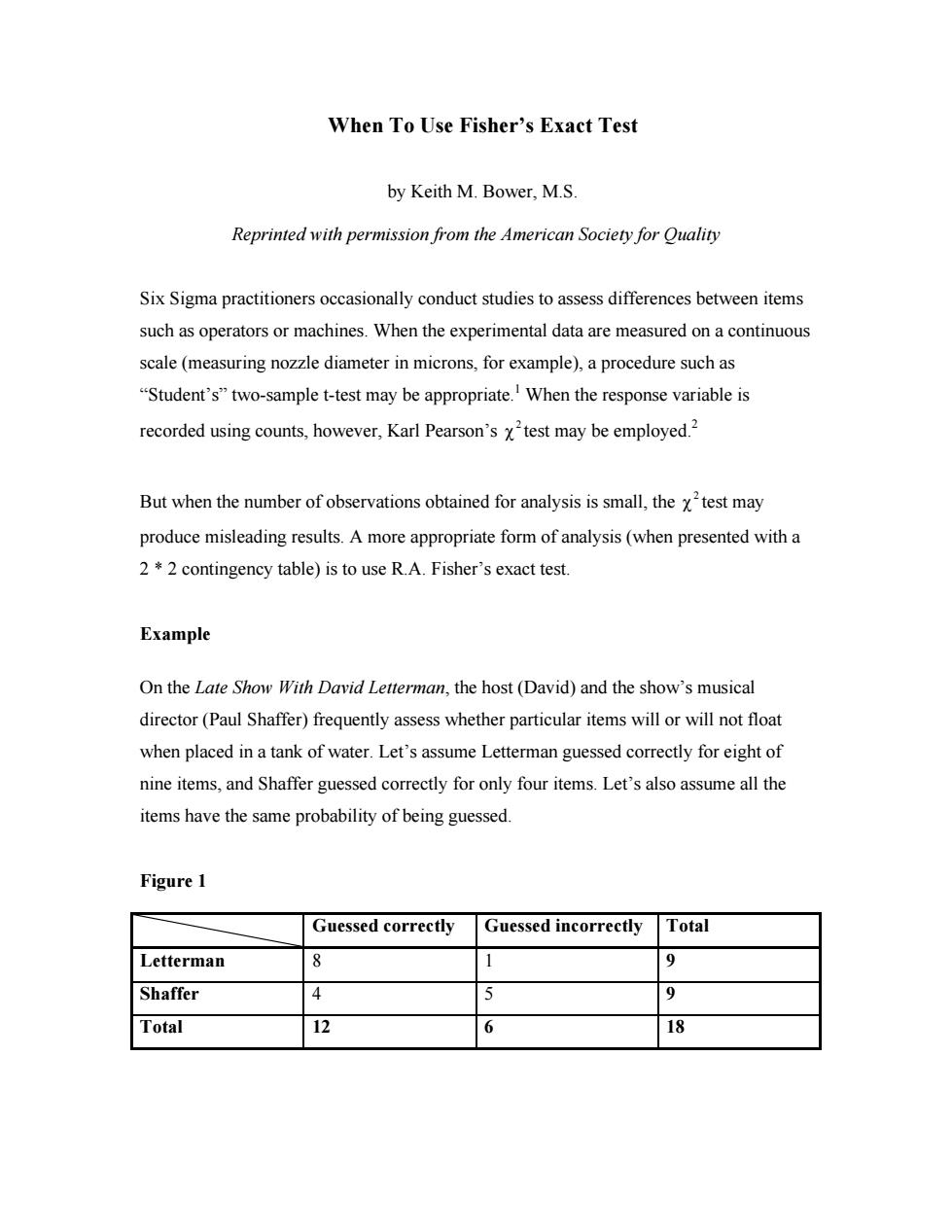
When To Use Fisher’s Exact Test by Keith M. Bower, M.S. Reprinted with permission from the American Society for Quality Six Sigma practitioners occasionally conduct studies to assess differences between items such as operators or machines. When the experimental data are measured on a continuous scale (measuring nozzle diameter in microns, for example), a procedure such as “Student’s” two-sample t-test may be appropriate.1 When the response variable is recorded using counts, however, Karl Pearson’s test may be employed. 2 χ 2 But when the number of observations obtained for analysis is small, the test may produce misleading results. A more appropriate form of analysis (when presented with a 2 * 2 contingency table) is to use R.A. Fisher’s exact test. 2 χ Example On the Late Show With David Letterman, the host (David) and the show’s musical director (Paul Shaffer) frequently assess whether particular items will or will not float when placed in a tank of water. Let’s assume Letterman guessed correctly for eight of nine items, and Shaffer guessed correctly for only four items. Let’s also assume all the items have the same probability of being guessed. Figure 1 Guessed correctly Guessed incorrectly Total Letterman 8 1 9 Shaffer 4 5 9 Total 12 6 18
You would typically use the x'test when presented with the contingency table results in Figure 1.In this case,the x'test assesses what the expected frequencies would be if the null hypothesis(equal proportions)was true.For example,if there were no difference between Letterman and Shaffer's guesses,you would expect Letterman to have been correct six times(see Figure 2).This is calculated as(9*12)/18=108/18=6. Figure 2 Rows:Player Columns:Result Correct Incorrect A11 David 8 1 9 6.00 3.00 9.00 Paul 4 5 9 6.00 3.00 9.00 A11 12 6 18 12.00 6.00 18.00 Chi-Square 4.000,DF 1,P-Value 0.046 2 cells with expected counts less than 5.0 Cell Contents-- Count Exp Freq The resulting p-value,0.046,from the x'test indicates there is a statistically significant difference (at the a=0.05 level)in the success rates between Letterman and Shaffer. As Fisher discusses,however,"The treatment of frequencies by means of x2 is an approximation,which is useful for the comparative simplicity of the calculations.The exact treatment is somewhat more laborious,though necessary in cases of doubt."3 Some practitioners will experience a problem when an expected value is less than five (this is what Fisher alludes to in his statement of doubt).Sometimes it's appropriate to group certain categories to avoid the problem,but this is clearly not possible when there are only two categories.As shown in Figure 2,there are two cells in which the expected counts are less than five
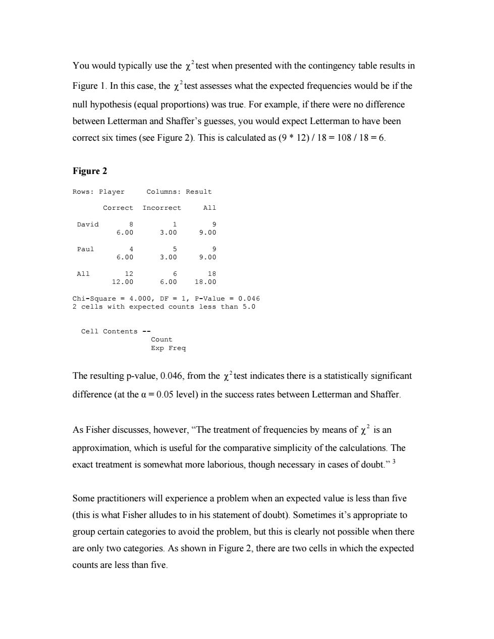
You would typically use the test when presented with the contingency table results in Figure 1. In this case, the test assesses what the expected frequencies would be if the null hypothesis (equal proportions) was true. For example, if there were no difference between Letterman and Shaffer’s guesses, you would expect Letterman to have been correct six times (see Figure 2). This is calculated as (9 * 12) / 18 = 108 / 18 = 6. 2 χ 2 χ Figure 2 Rows: Player Columns: Result Correct Incorrect All David 8 1 9 6.00 3.00 9.00 Paul 4 5 9 6.00 3.00 9.00 All 12 6 18 12.00 6.00 18.00 Chi-Square = 4.000, DF = 1, P-Value = 0.046 2 cells with expected counts less than 5.0 Cell Contents -- Count Exp Freq The resulting p-value, 0.046, from the test indicates there is a statistically significant difference (at the α = 0.05 level) in the success rates between Letterman and Shaffer. 2 χ As Fisher discusses, however, “The treatment of frequencies by means of is an approximation, which is useful for the comparative simplicity of the calculations. The exact treatment is somewhat more laborious, though necessary in cases of doubt.” 2 χ 3 Some practitioners will experience a problem when an expected value is less than five (this is what Fisher alludes to in his statement of doubt). Sometimes it’s appropriate to group certain categories to avoid the problem, but this is clearly not possible when there are only two categories. As shown in Figure 2, there are two cells in which the expected counts are less than five
Fisher's exact test considers all the possible cell combinations that would still result in the marginal frequencies as highlighted(namely 9,9 and 12,6).The test is exact because it uses the exact hypergeometric distribution rather than the approximate chi-square distribution to compute the p-value. The resulting p-value using Fisher's exact test is 0.1312.Therefore,you would fail to reject the null hypothesis of equal proportions at the a=0.05 level.This contradicts the results from the x'test and indicates the x'test provided a poor approximation to the exact results. The computations involved in Fisher's exact test may be extremely time consuming to calculate by hand,but are in the sidebar"Calculations for Fisher's Exact Test"for illustration.Clearly,it's much easier to use a statistical software package to obtain these results. Implications It's appropriate to use Fisher's exact test,in particular when dealing with small counts. The x2test is basically an approximation of the results from the exact test,so erroneous results could potentially be obtained from the few observations.This could lead to incorrect conclusions in Six Sigma projects. References 1.For more information on the two-sample t-test,see "The Two-Sample t-Test and Randomization Test"by Keith M.Bower,Six Sigma Forum,June 13,2003. 2.Karl Pearson,"On the Criterion That a Given System of Deviations From the Probable in the Case of Correlated System of Variables Is Such That It Can Be Reasonably Supposed To Have Arisen From Random Sampling,"Philosophical Magazine,Series V,No.1,(1900),pp.157-175
Fisher’s exact test considers all the possible cell combinations that would still result in the marginal frequencies as highlighted (namely 9, 9 and 12, 6). The test is exact because it uses the exact hypergeometric distribution rather than the approximate chi-square distribution to compute the p-value. The resulting p-value using Fisher’s exact test is 0.1312. Therefore, you would fail to reject the null hypothesis of equal proportions at the α = 0.05 level. This contradicts the results from the test and indicates the test provided a poor approximation to the exact results. 2 χ 2 χ The computations involved in Fisher’s exact test may be extremely time consuming to calculate by hand, but are in the sidebar “Calculations for Fisher’s Exact Test” for illustration. 4 Clearly, it’s much easier to use a statistical software package to obtain these results. Implications It’s appropriate to use Fisher’s exact test, in particular when dealing with small counts. The test is basically an approximation of the results from the exact test, so erroneous results could potentially be obtained from the few observations. This could lead to incorrect conclusions in Six Sigma projects. 2 χ References 1. For more information on the two-sample t-test, see “The Two-Sample t-Test and Randomization Test” by Keith M. Bower, Six Sigma Forum, June 13, 2003. 2. Karl Pearson, “On the Criterion That a Given System of Deviations From the Probable in the Case of Correlated System of Variables Is Such That It Can Be Reasonably Supposed To Have Arisen From Random Sampling,” Philosophical Magazine, Series V, No. 1, (1900), pp. 157-175
3.Ronald A.Fisher,Statistical Methods for Research Workers,14th edition,Hafner Publishing,1970,p.96. 4.To compute Fisher's exact test,refer to answer 210 at http://www.minitab.com/support/answers Bibliography Fleiss,Joseph L.,Statistical Methods for Rates and Proportions,John Wiley and Sons,1981 Montgomery,Douglas C.,and George C.Runger,Applied Statistics and Probability for Engineers,second edition,John Wiley and Sons,1999 SIDEBAR Calculations for Fisher's Exact Test The hypergeometric probability distribution is used to compute the probability of the observed results(see Table 1). Table 1 Correct Incorrect Total Letterman 8 1 9 Shaffer 4 5 9 Total 12 6 18 The remaining tables that will be consistent with the marginal frequencies of 9,9 and 12, 6,along with their associated probabilities,are shown in Table 2. To compute Fisher's exact test results,look at the tables with probabilities less than or equal to the probability of the observed results(0.061085972).They are highlighted with an *Add these probabilities together,along with the probability of the observed results, to obtain the p-value for the test
3. Ronald A. Fisher, Statistical Methods for Research Workers, 14th edition, Hafner Publishing, 1970, p. 96. 4. To compute Fisher’s exact test, refer to answer 210 at http://www.minitab.com/support/answers Bibliography Fleiss, Joseph L., Statistical Methods for Rates and Proportions, John Wiley and Sons, 1981. Montgomery, Douglas C., and George C. Runger, Applied Statistics and Probability for Engineers, second edition, John Wiley and Sons, 1999. SIDEBAR Calculations for Fisher’s Exact Test The hypergeometric probability distribution is used to compute the probability of the observed results (see Table 1). Table 1 Correct Incorrect Total Letterman 8 1 9 Shaffer 4 5 9 Total 12 6 18 The remaining tables that will be consistent with the marginal frequencies of 9, 9 and 12, 6, along with their associated probabilities, are shown in Table 2. To compute Fisher’s exact test results, look at the tables with probabilities less than or equal to the probability of the observed results (0.061085972). They are highlighted with an *. Add these probabilities together, along with the probability of the observed results, to obtain the p-value for the test
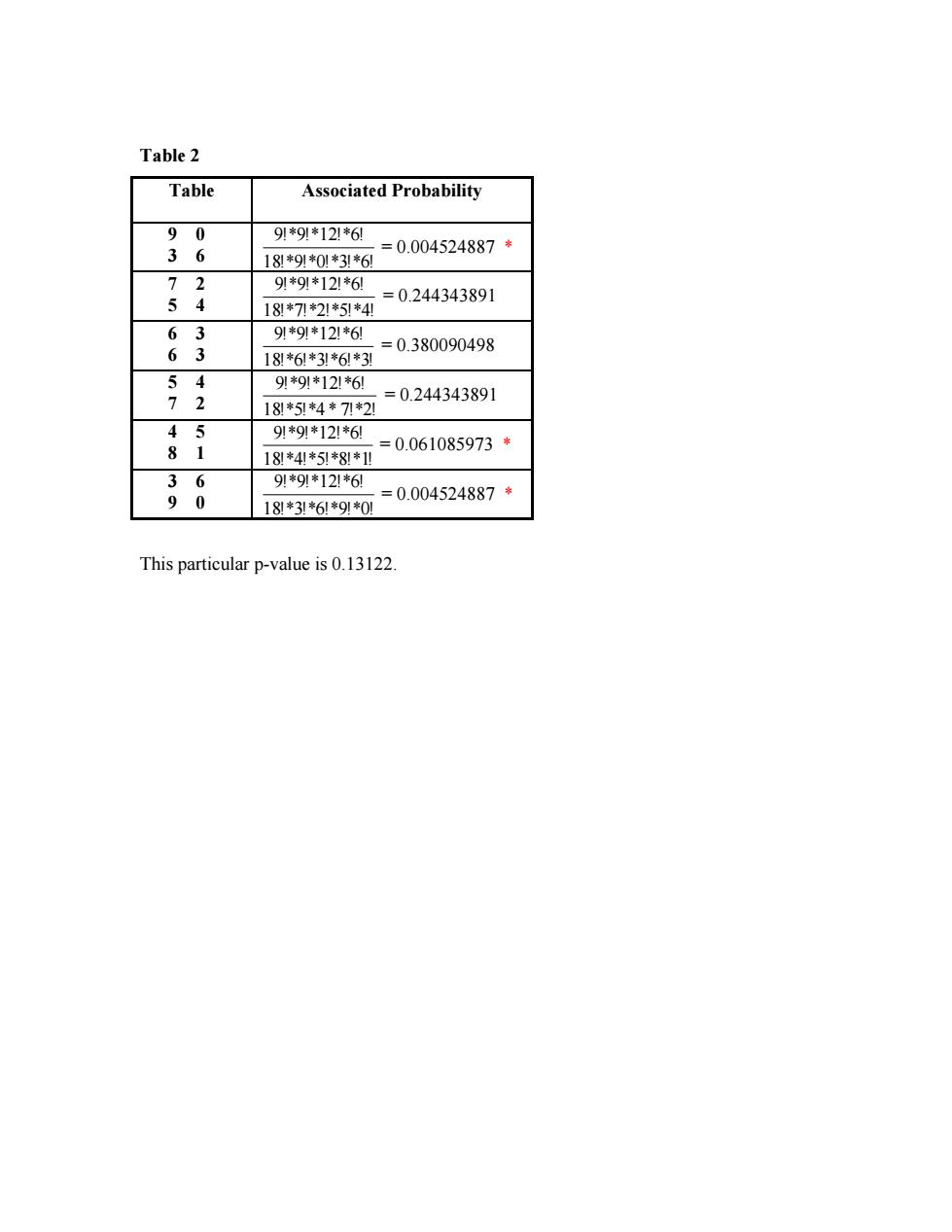
Table 2 Table Associated Probability 90 91*91*121*6) 36 =0.004524887* 181*91*01*31*61 72 91*91*121*61 54 =0.244343891 181*7刀*2*51*4纠 63 91*91*121*6l 63 =0.380090498 181*61*31*6!*3到 54 91*91*121*61 72 =0.244343891 181*51*4*71*2川 45 91*91*121*6 81 =0.061085973* 181*41*51*81*1川 36 9列*9列*12!*6l 90 =0.004524887* 181*31*61*91*01 This particular p-value is 0.13122
Table 2 Table Associated Probability 9 0 3 6 18!*9!*0!*3!*6! 9!*9!*12!*6! = 0.004524887 * 7 2 5 4 18!*7!*2!*5!*4! 9!*9!*12!*6! = 0.244343891 6 3 6 3 18!*6!*3!*6!*3! 9!*9!*12!*6! = 0.380090498 5 4 7 2 18!*5!*4 * 7!*2! 9!*9!*12!*6! = 0.244343891 4 5 8 1 18!*4!*5!*8!*1! 9!*9!*12!*6! = 0.061085973 * 3 6 9 0 18!*3!*6!*9!*0! 9!*9!*12!*6! = 0.004524887 * This particular p-value is 0.13122