6 structures for discrete-time system 6.0 Introduction 6.1 Block Diagram Representation of Linear Constant-Coefficient Difference Equations 6.2 Signal Flow Graph Representation of Linear Constant-Coefficient Difference Equations 6.3 Basic Structures for IIR Systems 6.4 Transposed(转置)Forms 6.5 Basic Network Structures for FIR Systems 2
2 6.0 Introduction 6.1 Block Diagram Representation of Linear Constant-Coefficient Difference Equations 6.2 Signal Flow Graph Representation of Linear Constant-Coefficient Difference Equations 6.3 Basic Structures for IIR Systems 6.4 Transposed(转置) Forms 6.5 Basic Network Structures for FIR Systems §6 structures for discrete-time system
Structures for Discrete-Time Systems 6.0 Introduction 3
3 Structures for Discrete-Time Systems 6.0 Introduction

6.0 Introduction Characterization of an LTI System: ◆Impulse Response h[n]→Frequency response z-Transform:system function H(=)= b+bzY(=) 1-azX(2) Difference Equation yn]ayn1]xx1] converted to a algorithm or structure that can be realized in the desired technology, when implemented with hardware. Structure consists of an interconnection of basic operations of addition,multiplication by a constant and delay 4
4 Characterization of an LTI System: ◆Impulse Response h[n] ◆z-Transform: system function ◆Difference Equation ◆converted to a algorithm or structure that can be realized in the desired technology, when implemented with hardware. ◆Structure consists of an interconnection of basic operations of addition, multiplication by a constant and delay 6.0 Introduction → Frequency response 1 0 1 1 ( ) 1 ( ) ( ) b bz H z az Y z X z − − + = − = y n ay n b x n bx n − − = + − 1 1 0 1
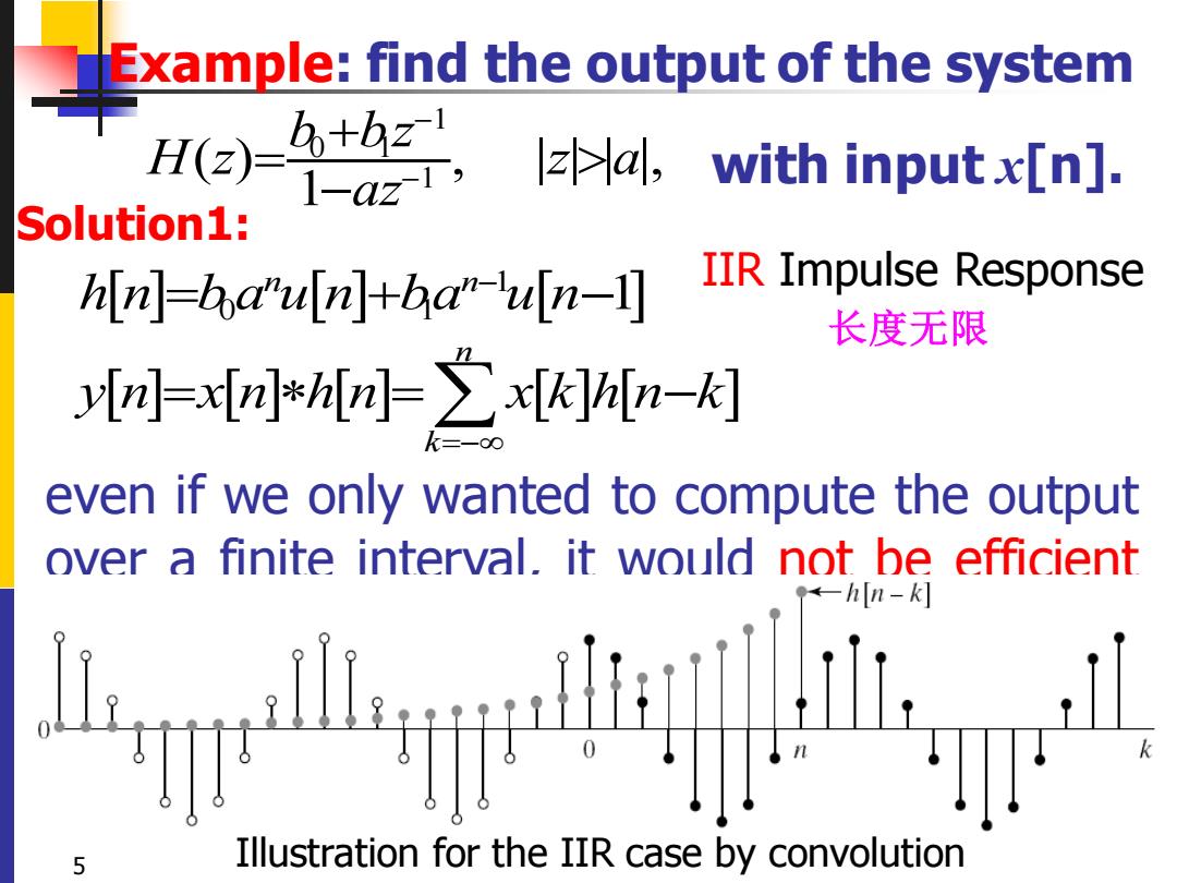
Example:find the output of the system H(z)= b+b2 I-az-T a,with input x[n]. Solution1: hin]=ha"uln]+ba"-uln-I] IIR Impulse Response 长度无限 yIri]=x[n]*hr]=x[k]hn-k] even if we only wanted to compute the output over a finite interval.it would not be efficient h n-k Illustration for the IIR case by convolution
with input x[n]. even if we only wanted to compute the output over a finite interval, it would not be efficient to do so by discrete convolution, since the amount of computation required to compute y[n] would grow with n . 5 1 0 1 1 ( ) , | | | |, 1 b bz H z z a az − − + = − 1 0 1 1 n n h n b a u n ba u n − = + − n k y n x n h n x k h n k =− = = − Illustration for the IIR case by convolution IIR Impulse Response 长度无限 Example: find the output of the system Solution1:

Example:find the output of the system 1H(z)= b+bzY(z) 1-azX(2) a,with input x[n]. Solution2: yIn]ayln 1]=bxn]bxIn I] yn=ay n-Iaxn+bxn-1 causal LTI 递推计算recursive computation of output(unique?) using only y n-1,xn,x n-1]. initial-rest conditions(for n<nor if x[n]=0,then y[n]=0 The algorithm suggested by the equation is not the only computational algorithm,there are unlimited variety of computational structures (shown later)
with input x[n]. 6 Example: find the output of the system 1 0 1 1 ( ) , | | | |, 1 ( ) ( ) b bz H z z a az Y z X z − − = + = − y n ay n b x n bx n − − = + − 1 1 0 1 y n ay n b x n bx n = − + + − 1 1 0 1 recursive computation of output (unique?) using only y[n-1], x[n], x[n-1]. The algorithm suggested by the equation is not the only computational algorithm, there are unlimited variety of computational structures (shown later). Solution2: initial-rest conditions(for n<n0 , if x[n]=0, then y[n]=0) causal LTI 递推计算

Why Implement system Using Different Structures? Equivalent structures with regard to their input-output characteristics for infinite-precision representation,may have vastly different behavior when numerical precision is limited. Computational structures(Modeling methods): ◆Block Diagram ◆Signal Flow Graph 7
7 Why Implement system Using Different Structures? ◆Equivalent structures with regard to their input-output characteristics for infinite-precision representation, may have vastly different behavior when numerical precision is limited. ◆Computational structures(Modeling methods): ◆Block Diagram ◆Signal Flow Graph
Structures for Discrete-Time Systems 6.1 Block Diagram Representation of Linear Constant-Coefficient Difference Equations 8
8 Structures for Discrete-Time Systems 6.1 Block Diagram Representation of Linear Constant-Coefficient Difference Equations
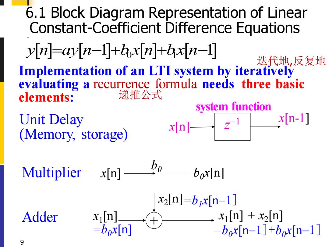
6.1 Block Diagram Representation of Linear Constant-Coefficient Difference Equations yIn]=ayIn-I]axInj+axIn-1] 迭代地,反复地 Implementation of an lTI system by iteratively evaluating a recurrence formula needs three basic elements: 递推公式 system function Unit Delay x[n] x[n-1] (Memory,storage) Multiplier x[n] bo x2[n]=bx[n-1] Adder x1[n] x[n]+x2[n] =boxIn] =bx[n-1]+bx[n-1] 9
9 6.1 Block Diagram Representation of Linear Constant-Coefficient Difference Equations + x1 [n] x2 [n] x1 [n] + x2 Adder [n] x[n] b0 Multiplier b0x[n] x[n] x[n-1] z Unit Delay −1 (Memory, storage) y n ay n b x n bx n = − + + − 1 1 0 1 Implementation of an LTI system by iteratively evaluating a recurrence formula needs three basic elements: M sample system function 递推公式 =b0x[n] =b1x[n−1] =b0x[n−1]+b0x[n−1] 迭代地,反复地

Ex.6.1 draw Block Diagram Representation of a Second-order Difference Equation Mn]=ayn-I]+ayIn-2]+axn] [n]-aMn-l]-4[n-2]=b[n] Solution: x[n] bo y(n] y(n] Y(z)b X(z)1-4z1-4z y(n-1] =H(z) 02 y[n-2] 10
10 Ex. 6.1 draw Block Diagram Representation of a Second-order Difference Equation 1 2 0 y n y n y n b x n [ ] [ 1] [ 2] [ ] = − + − + a a + a1 a2 y[n] y[n-1] y[n-2] 0 2 1 2 1 ( ) ( ) 1 Y z b X z a z a z − − − − = Solution: =H z( ) 1 2 0 y n y n y n b x n [ ] [ 1] [ 2] [ ] − − a a − − = z −1 z −1 y[n] x[n] + b0

Nth-Order Difference Equations change M Equation to a儿n-k]=∑bx[n-k] = =0 k=0 M normalized y儿川-∑aMn-k]=∑bx[n-k] to unity k=1 k=03 [川]=之aHn-k]+之,m-k利 M k=1 k=0 M H(z)= k=0 11
11 Nth-Order Difference Equations 1 0 [ ] [ ] [ ] = = − − = − N k k k k M y n y n k n k a b x ( ) 0 1 1 M k k k N k k k b z H z a z − = − = − = 0 0 [ ] [ ] N k k M k k a y n k x k b n = = − = − 1 0 [ ] [ ] [ ] N M k k k k y n a y n k b x n k = = = − + − change Equation to a’ 0 normalized to unity 0 0 [ ] [ ] N M k k k k a y n k b x n k = = − = −