
First-Cut Techniques The Greedy Approach Graph Traversal A common characteristic of both greedy algorithms and graph traversal is that they are fast,as they involve making local decisions
First-Cut Techniques ◼ The Greedy Approach ◼ Graph Traversal ⚫ A common characteristic of both greedy algorithms and graph traversal is that they are fast, as they involve making local decisions
The Greedy Approach As in the case of dynamic programming algorithms, greedy algorithms are usually designed to solve optimization problems in which a quantity is to be minimized or maximized. Unlike dynamic programming algorithms,greedy algorithms typically consist of a n iterative procedure that tries to find a local optimal solution. In some instances,these local optimal solutions translate to global optimal solutions.In others,they fail to give optimal solutions
The Greedy Approach ◼ As in the case of dynamic programming algorithms, greedy algorithms are usually designed to solve optimization problems in which a quantity is to be minimized or maximized. ◼ Unlike dynamic programming algorithms, greedy algorithms typically consist of a n iterative procedure that tries to find a local optimal solution. ◼ In some instances, these local optimal solutions translate to global optimal solutions. In others, they fail to give optimal solutions
The Greedy Approach A greedy algorithm makes a correct guess on the basis of little calculation without worrying about the future.Thus,it builds a solution step by step.Each step increases the size of the partial solution and is based on local optimization. The choice make is that which produces the /argest immediate gain while maintaining feasibility. ■ Since each step consists of little work based on a small amount of information,the resulting algorithms are typically efficient
The Greedy Approach ◼ A greedy algorithm makes a correct guess on the basis of little calculation without worrying about the future. Thus, it builds a solution step by step. Each step increases the size of the partial solution and is based on local optimization. ◼ The choice make is that which produces the largest immediate gain while maintaining feasibility. ◼ Since each step consists of little work based on a small amount of information, the resulting algorithms are typically efficient
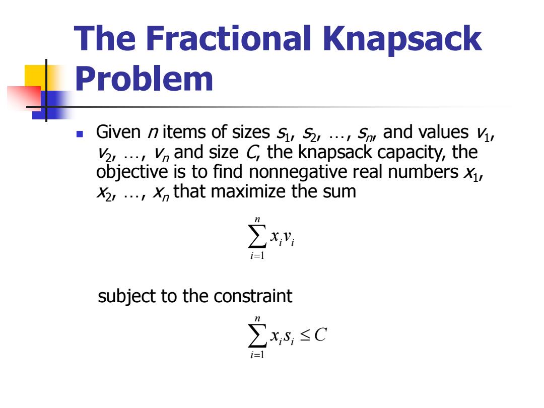
The Fractional Knapsack Problem Given n items of sizes s,s,...,s and values v, v,...,and size C the knapsack capacity,the objective is to find nonnegative real numbers, X2,...,that maximize the sum i=1 subject to the constraint ∑xs,≤C i=1
The Fractional Knapsack Problem ◼ Given n items of sizes s1 , s2 , …, sn , and values v1 , v2 , …, vn and size C, the knapsack capacity, the objective is to find nonnegative real numbers x1 , x2 , …, xn that maximize the sum = n i i i x v 1 = n i xi si C 1 subject to the constraint
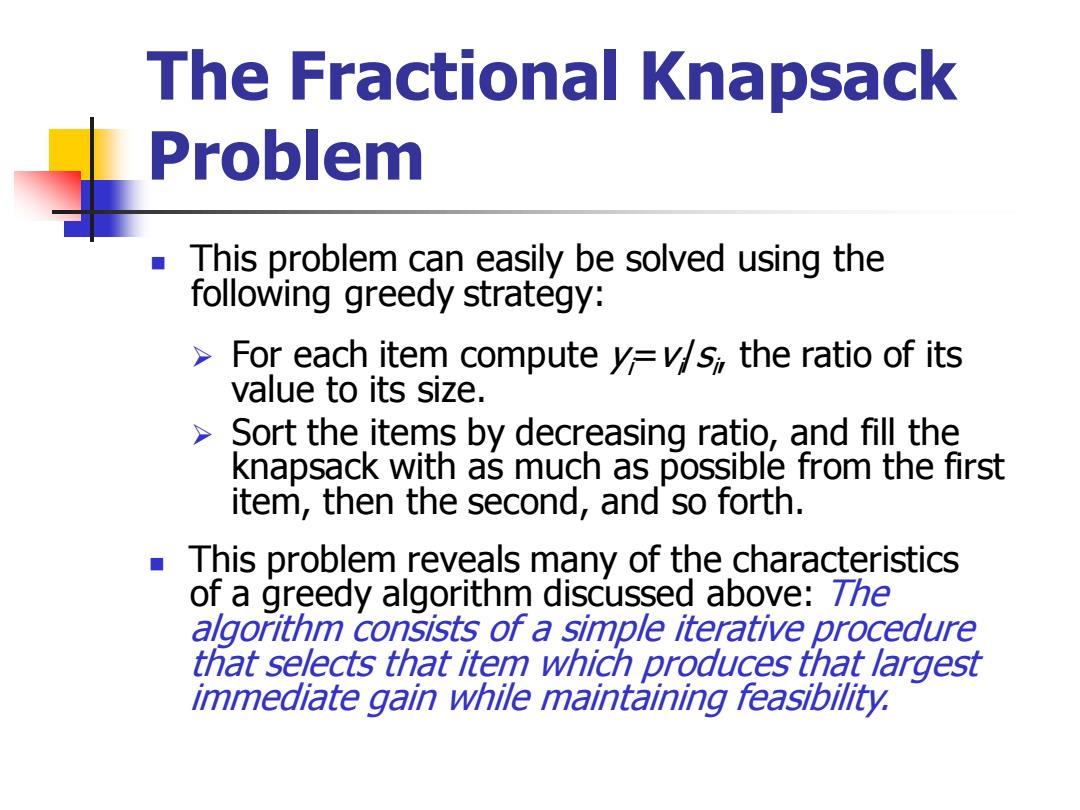
The Fractional Knapsack Problem This problem can easily be solved using the following greedy strategy: For each item computey=/s the ratio of its value to its size. Sort the items by decreasing ratio,and fill the knapsack with as much as possible from the first item,then the second,and so forth. This problem reveals many of the characteristics of a greedy algorithm discussed above:7he algorithm consists of a simple iterative procedure that selects that item which produces that largest immediate gain while maintaining feasibility
The Fractional Knapsack Problem ◼ This problem can easily be solved using the following greedy strategy: ➢ For each item compute yi=vi /si , the ratio of its value to its size. ➢ Sort the items by decreasing ratio, and fill the knapsack with as much as possible from the first item, then the second, and so forth. ◼ This problem reveals many of the characteristics of a greedy algorithm discussed above: The algorithm consists of a simple iterative procedure that selects that item which produces that largest immediate gain while maintaining feasibility
The Shortest Path Problem ● Let G=(,E)be a directed graph in which each edge has a nonnegative length,and a distinguished vertex s called the source.The single-source shortest path problem,or simply the shortest path problem,is to determine the distance from s to every other vertex in where the distance from vertex s to vertex xis defined as the length of a shortest path from sto x. For simplicity,we will assume that V1,2,...,n) and s=1. This problem can be solved using a greedy technique known as Dijkstra's algorithm
The Shortest Path Problem ◼ Let G=(V, E) be a directed graph in which each edge has a nonnegative length, and a distinguished vertex s called the source. The single-source shortest path problem, or simply the shortest path problem, is to determine the distance from s to every other vertex in V, where the distance from vertex s to vertex x is defined as the length of a shortest path from s to x. ◼ For simplicity, we will assume that V={1, 2, …, n} and s=1. ◼ This problem can be solved using a greedy technique known as Dijkstra’s algorithm
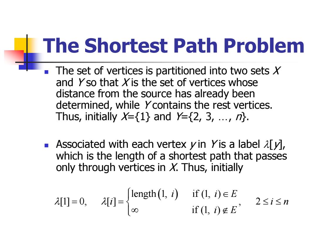
The Shortest Path Problem The set of vertices is partitioned into two sets x and yso that Xis the set of vertices whose distance from the source has already been determined,while ycontains the rest vertices. Thus,initially =1}and Y=2,3,...,n. Associated with each vertex yin Yis a label[☑, which is the length of a shortest path that passes only through vertices in X.Thus,initially if(L,i)∈E 0=0, 2≤i≤n if(1,iE
The Shortest Path Problem ◼ The set of vertices is partitioned into two sets X and Y so that X is the set of vertices whose distance from the source has already been determined, while Y contains the rest vertices. Thus, initially X={1} and Y={2, 3, …, n}. ◼ Associated with each vertex y in Y is a label [y], which is the length of a shortest path that passes only through vertices in X. Thus, initially length 1, if (1, ) ( ) [1] 0, [ ] , 2 if (1, ) i i E i i n i E = =
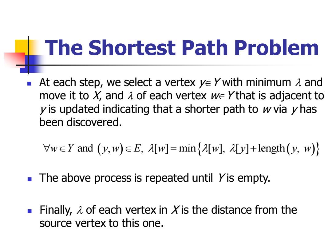
The Shortest Path Problem a At each step,we select a vertex ve ywith minimum 1 and move it to x,and a of each vertex we ythat is adjacent to yis updated indicating that a shorter path to wvia yhas been discovered. VwEY and (y,w)EE,[w]=min(w],y]+length(y,w) The above process is repeated until Yis empty. Finally,1 of each vertex in Xis the distance from the source vertex to this one
The Shortest Path Problem ◼ At each step, we select a vertex yY with minimum and move it to X, and of each vertex wY that is adjacent to y is updated indicating that a shorter path to w via y has been discovered. = + w Y y w E w w y y w and , , [ ] min [ ], [ ] length , ( ) ( ) ◼ The above process is repeated until Y is empty. ◼ Finally, of each vertex in X is the distance from the source vertex to this one
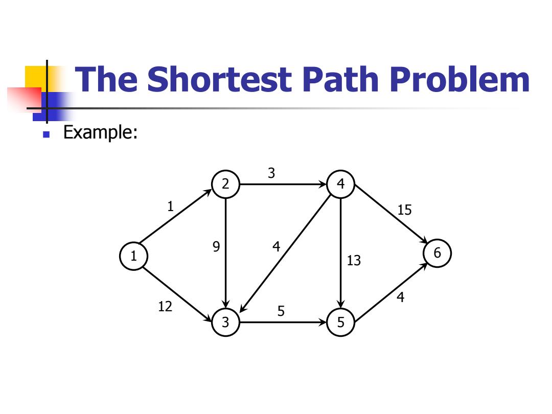
The Shortest Path Problem Example: 3 2 4 1 15 9 4 1 13 6 4 12 5 3 5
The Shortest Path Problem ◼ Example: 1 2 3 4 5 6 1 12 9 3 4 5 13 15 4
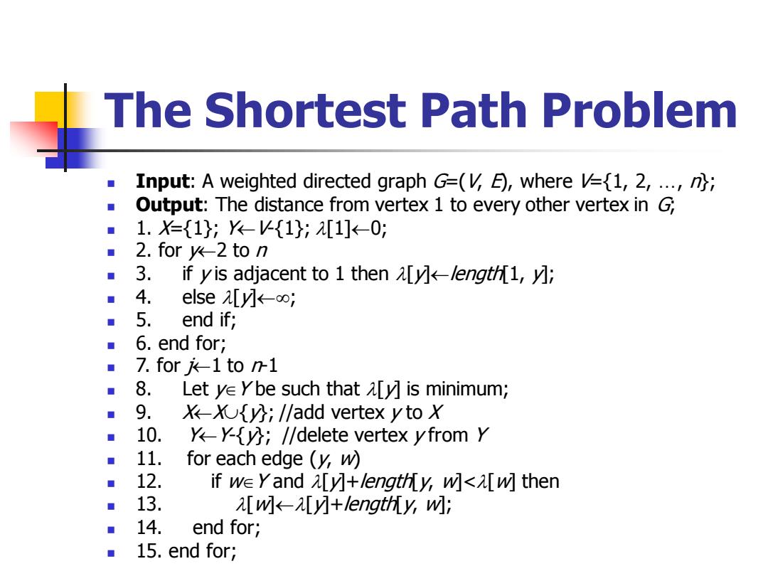
The Shortest Path Problem Input:A weighted directed graph G=(E),where V1,2,...,; Output:The distance from vertex 1 to every other vertex in G; 1.={1;-{1;[1]←-0; ■ 2.for v2 to n ■ 3. if yis adjacent to1 then 2[☑k--length1,☑; ■ 4. else [y☑k-o; ■ 5. end if; 6.end for; 7.for六-1tor1 ■ 8. Let ye ybe such that a[y]is minimum; 9. Xxoy);//add vertex ytoX 10. Yy);//delete vertex yfrom Y 11. for each edge (y,w) 12. if we Yand i[y]+lengthly,w]<a[w]then 13. 2[M←-[☑+ength[y,WM: 14 end for; ■ 15. end for;
The Shortest Path Problem ◼ Input: A weighted directed graph G=(V, E), where V={1, 2, …, n}; ◼ Output: The distance from vertex 1 to every other vertex in G; ◼ 1. X={1}; YV-{1}; [1]0; ◼ 2. for y2 to n ◼ 3. if y is adjacent to 1 then [y]length[1, y]; ◼ 4. else [y]; ◼ 5. end if; ◼ 6. end for; ◼ 7. for j1 to n-1 ◼ 8. Let yY be such that [y] is minimum; ◼ 9. XX{y}; //add vertex y to X ◼ 10. YY-{y}; //delete vertex y from Y ◼ 11. for each edge (y, w) ◼ 12. if wY and [y]+length[y, w]<[w] then ◼ 13. [w][y]+length[y, w]; ◼ 14. end for; ◼ 15. end for;