[Go back to CEM 333 Course Information Page][Go back to CEM 333 Home Page] An Excel Spreadsheet Exercise* Question Use the data in the table below to construct a spreadsheet showing the titration curve data, the first-derivative data and the second-derivative data. Plot each of these results versus titrant volume and determine the end point of the titration. Volume AgNO3, mL E vs. SCE, V 5.00 0.062 15.00 0.085 20.00 0.107 22.00 0.123 24.00 0.138 23.50 0.146 23.80 0.161 24.00 0.174 24.10 0.183 24.20 0.194 24.30 0.233 24.40 0.316 24.50 0.340 24.60 0.351 24.70 0.358
[Go back to CEM 333 Course Information Page][Go back to CEM 333 Home Page] An Excel Spreadsheet Exercise* Question Use the data in the table below to construct a spreadsheet showing the titration curve data, the first-derivative data and the second-derivative data. Plot each of these results versus titrant volume and determine the end point of the titration. Volume AgNO3, mL E vs. SCE, V 5.00 0.062 15.00 0.085 20.00 0.107 22.00 0.123 24.00 0.138 23.50 0.146 23.80 0.161 24.00 0.174 24.10 0.183 24.20 0.194 24.30 0.233 24.40 0.316 24.50 0.340 24.60 0.351 24.70 0.358
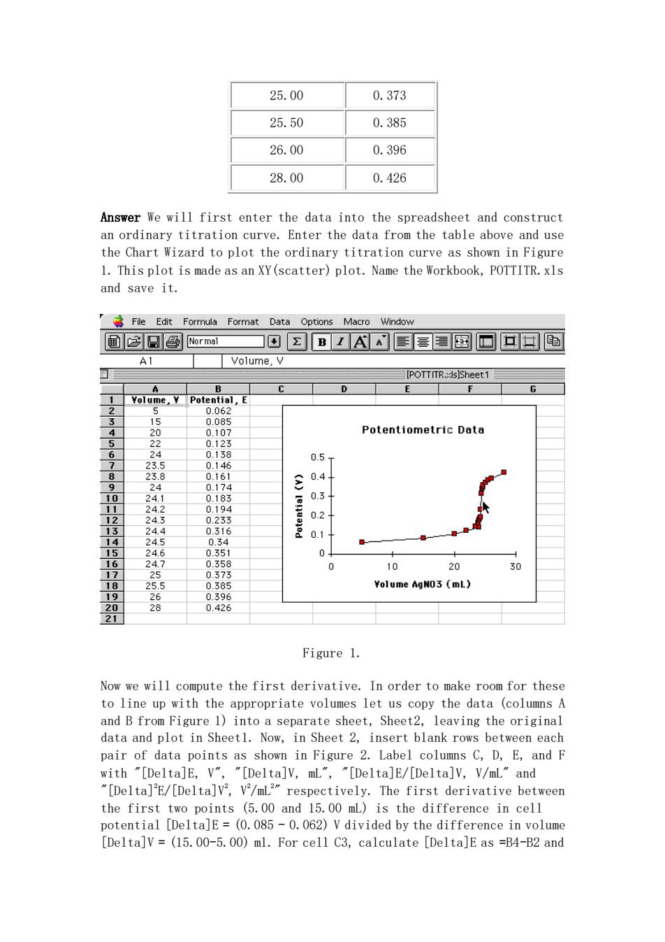
25.00 0.373 25.50 0.385 26.00 0.396 28.00 0.426 Answer We will first enter the data into the spreadsheet and construct an ordinary titration curve. Enter the data from the table above and use the Chart Wizard to plot the ordinary titration curve as shown in Figure 1. This plot is made as an XY(scatter) plot. Name the Workbook, POTTITR.xls and save it. Figure 1. Now we will compute the first derivative. In order to make room for these to line up with the appropriate volumes let us copy the data (columns A and B from Figure 1) into a separate sheet, Sheet2, leaving the original data and plot in Sheet1. Now, in Sheet 2, insert blank rows between each pair of data points as shown in Figure 2. Label columns C, D, E, and F with "[Delta]E, V", "[Delta]V, mL", "[Delta]E/[Delta]V, V/mL" and "[Delta]2 E/[Delta]V2 , V2 /mL2 " respectively. The first derivative between the first two points (5.00 and 15.00 mL) is the difference in cell potential [Delta]E = (0.085 - 0.062) V divided by the difference in volume [Delta]V = (15.00-5.00) ml. For cell C3, calculate [Delta]E as =B4-B2 and
25.00 0.373 25.50 0.385 26.00 0.396 28.00 0.426 Answer We will first enter the data into the spreadsheet and construct an ordinary titration curve. Enter the data from the table above and use the Chart Wizard to plot the ordinary titration curve as shown in Figure 1. This plot is made as an XY(scatter) plot. Name the Workbook, POTTITR.xls and save it. Figure 1. Now we will compute the first derivative. In order to make room for these to line up with the appropriate volumes let us copy the data (columns A and B from Figure 1) into a separate sheet, Sheet2, leaving the original data and plot in Sheet1. Now, in Sheet 2, insert blank rows between each pair of data points as shown in Figure 2. Label columns C, D, E, and F with "[Delta]E, V", "[Delta]V, mL", "[Delta]E/[Delta]V, V/mL" and "[Delta]2 E/[Delta]V2 , V2 /mL2 " respectively. The first derivative between the first two points (5.00 and 15.00 mL) is the difference in cell potential [Delta]E = (0.085 - 0.062) V divided by the difference in volume [Delta]V = (15.00-5.00) ml. For cell C3, calculate [Delta]E as =B4-B2 and
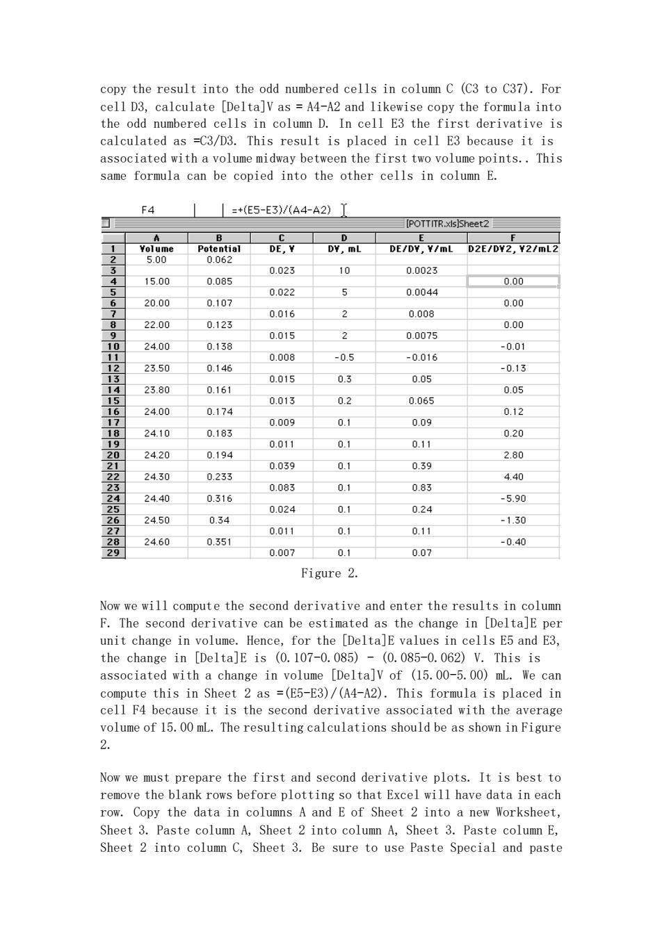
copy the result into the odd numbered cells in column C (C3 to C37). For cell D3, calculate [Delta]V as = A4-A2 and likewise copy the formula into the odd numbered cells in column D. In cell E3 the first derivative is calculated as =C3/D3. This result is placed in cell E3 because it is associated with a volume midway between the first two volume points. This same formula can be copied into the other cells in column E. Figure 2. Now we will compute the second derivative and enter the results in column F. The second derivative can be estimated as the change in [Delta]E per unit change in volume. Hence, for the [Delta]E values in cells E5 and E3, the change in [Delta]E is (0.107-0.085) - (0.085-0.062) V. This is associated with a change in volume [Delta]V of (15.00-5.00) mL. We can compute this in Sheet 2 as =(E5-E3)/(A4-A2). This formula is placed in cell F4 because it is the second derivative associated with the average volume of 15.00 mL. The resulting calculations should be as shown in Figure 2. Now we must prepare the first and second derivative plots. It is best to remove the blank rows before plotting so that Excel will have data in each row. Copy the data in columns A and E of Sheet 2 into a new Worksheet, Sheet 3. Paste column A, Sheet 2 into column A, Sheet 3. Paste column E, Sheet 2 into column C, Sheet 3. Be sure to use Paste Special and paste
copy the result into the odd numbered cells in column C (C3 to C37). For cell D3, calculate [Delta]V as = A4-A2 and likewise copy the formula into the odd numbered cells in column D. In cell E3 the first derivative is calculated as =C3/D3. This result is placed in cell E3 because it is associated with a volume midway between the first two volume points. This same formula can be copied into the other cells in column E. Figure 2. Now we will compute the second derivative and enter the results in column F. The second derivative can be estimated as the change in [Delta]E per unit change in volume. Hence, for the [Delta]E values in cells E5 and E3, the change in [Delta]E is (0.107-0.085) - (0.085-0.062) V. This is associated with a change in volume [Delta]V of (15.00-5.00) mL. We can compute this in Sheet 2 as =(E5-E3)/(A4-A2). This formula is placed in cell F4 because it is the second derivative associated with the average volume of 15.00 mL. The resulting calculations should be as shown in Figure 2. Now we must prepare the first and second derivative plots. It is best to remove the blank rows before plotting so that Excel will have data in each row. Copy the data in columns A and E of Sheet 2 into a new Worksheet, Sheet 3. Paste column A, Sheet 2 into column A, Sheet 3. Paste column E, Sheet 2 into column C, Sheet 3. Be sure to use Paste Special and paste
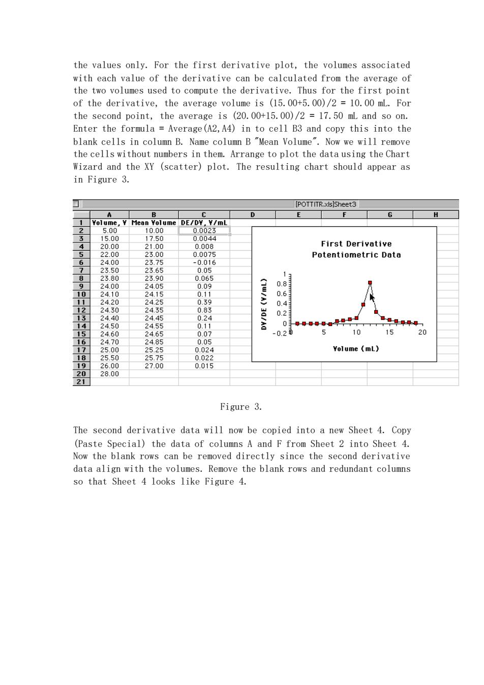
the values only. For the first derivative plot, the volumes associated with each value of the derivative can be calculated from the average of the two volumes used to compute the derivative. Thus for the first point of the derivative, the average volume is (15.00+5.00)/2 = 10.00 mL. For the second point, the average is (20.00+15.00)/2 = 17.50 mL and so on. Enter the formula = Average(A2,A4) in to cell B3 and copy this into the blank cells in column B. Name column B "Mean Volume". Now we will remove the cells without numbers in them. Arrange to plot the data using the Chart Wizard and the XY (scatter) plot. The resulting chart should appear as in Figure 3. Figure 3. The second derivative data will now be copied into a new Sheet 4. Copy (Paste Special) the data of columns A and F from Sheet 2 into Sheet 4. Now the blank rows can be removed directly since the second derivative data align with the volumes. Remove the blank rows and redundant columns so that Sheet 4 looks like Figure 4
the values only. For the first derivative plot, the volumes associated with each value of the derivative can be calculated from the average of the two volumes used to compute the derivative. Thus for the first point of the derivative, the average volume is (15.00+5.00)/2 = 10.00 mL. For the second point, the average is (20.00+15.00)/2 = 17.50 mL and so on. Enter the formula = Average(A2,A4) in to cell B3 and copy this into the blank cells in column B. Name column B "Mean Volume". Now we will remove the cells without numbers in them. Arrange to plot the data using the Chart Wizard and the XY (scatter) plot. The resulting chart should appear as in Figure 3. Figure 3. The second derivative data will now be copied into a new Sheet 4. Copy (Paste Special) the data of columns A and F from Sheet 2 into Sheet 4. Now the blank rows can be removed directly since the second derivative data align with the volumes. Remove the blank rows and redundant columns so that Sheet 4 looks like Figure 4
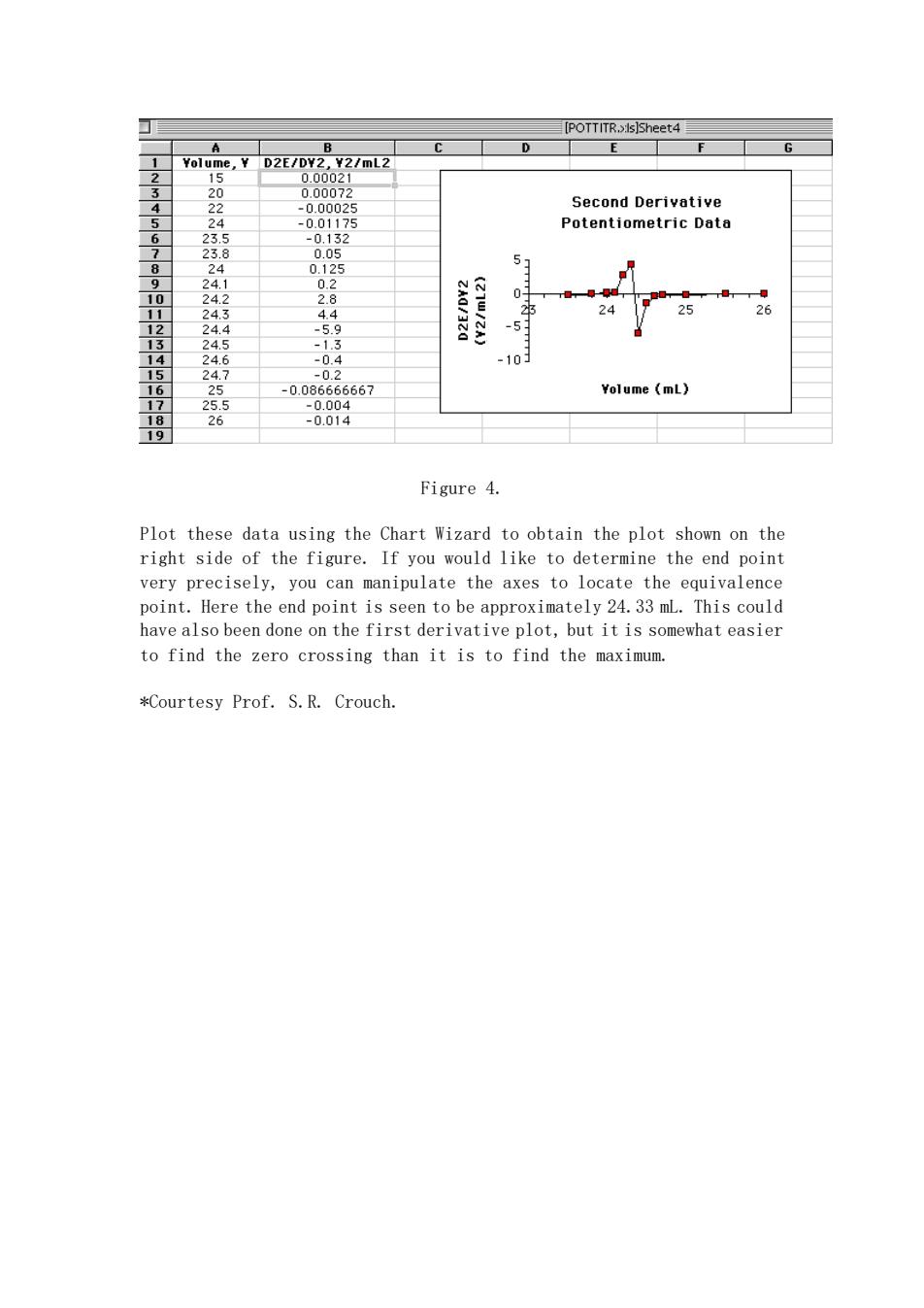
Figure 4. Plot these data using the Chart Wizard to obtain the plot shown on the right side of the figure. If you would like to determine the end point very precisely, you can manipulate the axes to locate the equivalence point. Here the end point is seen to be approximately 24.33 mL. This could have also been done on the first derivative plot, but it is somewhat easier to find the zero crossing than it is to find the maximum. *Courtesy Prof. S.R. Crouch
Figure 4. Plot these data using the Chart Wizard to obtain the plot shown on the right side of the figure. If you would like to determine the end point very precisely, you can manipulate the axes to locate the equivalence point. Here the end point is seen to be approximately 24.33 mL. This could have also been done on the first derivative plot, but it is somewhat easier to find the zero crossing than it is to find the maximum. *Courtesy Prof. S.R. Crouch