
Chapter 11 Estimation of Specific Parameters UESTC 1
1 UESTC Chapter 11 Estimation of Specific Parameters
11.1 Chapter highlights Parameter estimation in WGN Amplitude estimation in the coherent case Amplitude estimation in the noncoherent case Phase estimation in WGN Time-delay estimation in WGN Frequency estimation in WGN UESTC 2
2 UESTC 11.1 Chapter highlights • Parameter estimation in WGN • Amplitude estimation in the coherent case • Amplitude estimation in the noncoherent case • Phase estimation in WGN • Time-delay estimation in WGN • Frequency estimation in WGN
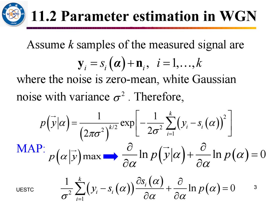
11.2 Parameter estimation in WGN Assume k samples of the measured signal are y;=s;(a)+n,i=1,...,k where the noise is zero-mean,white Gaussian noise with variance o2.Therefore, 心e7齐-ej MAP.p可mx→p(ik)+小&np(a)-0 UESTC 是立(g-aa@+npa=0
11.2 Parameter estimation in WGN Assume k samples of the measured signal are where the noise is zero-mean, white Gaussian noise with variance . Therefore, MAP: 3 UESTC ( ) , 1, , i i i y n = + = s i k α 2 ( ) ( ) ( ( )) 2 / 2 2 2 1 1 1 exp 2 2 k k i i i p y y s = = − − ln ln 0 p y p ( ) ( ) + = p y ( ) max ( ( )) ( ) ( ) 2 1 1 ln 0 k i i i i s y s p = − + =
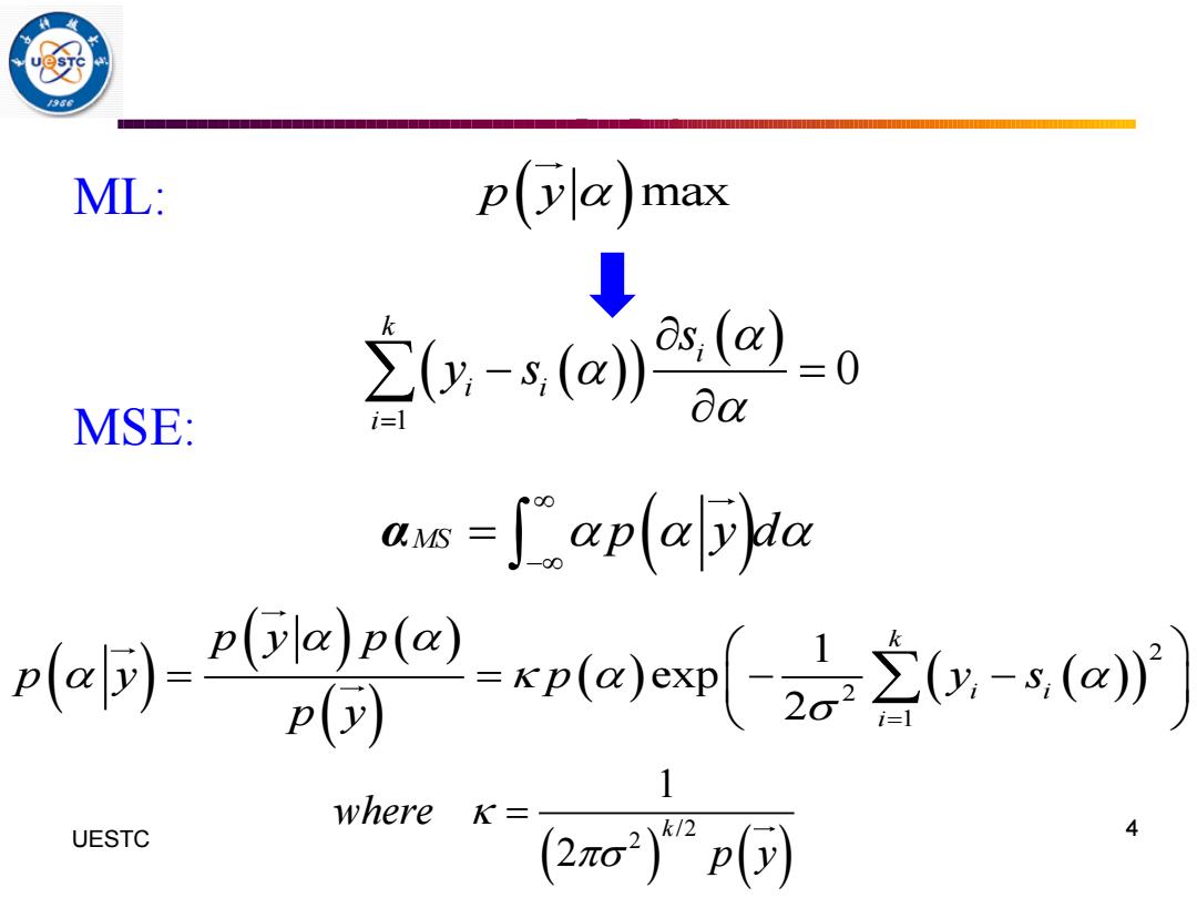
ML: p(a max 20x-sj)22-0 MSE: na as-aplaya e同-4 d 1 where K= UESTC 2o2p可 4
ML: MSE: 4 UESTC p y( )max ( ( )) ( ) 1 0 k i i i i s y s = − = MS p y d ( ) − = α ( ) ( ) ( ) ( ) ( ) ( ( ))2 2 1 1 exp 2 k i i i p y p p y p y s p y = = = − − ( ) ( ) / 2 2 1 2 where k p y =
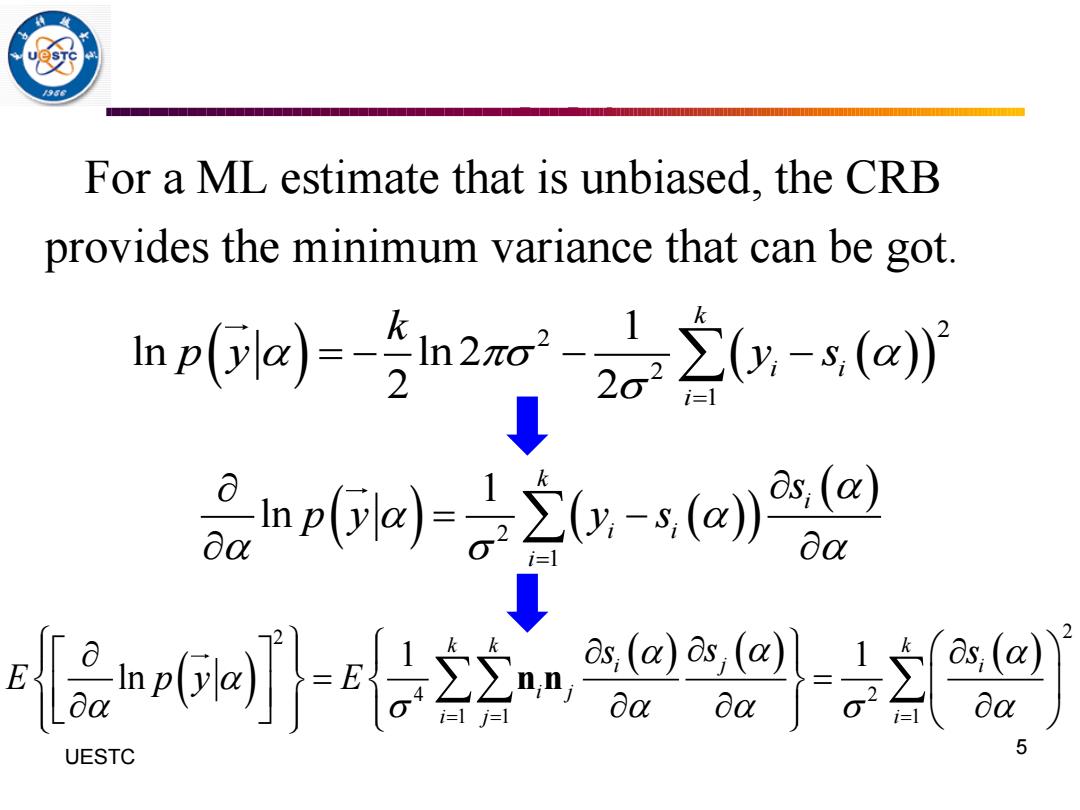
5 For a ML estimate that is unbiased,the CRB provides the minimum variance that can be got. npa)-n2ar-2a立(ysai i1 品mp啡a之yag I- ↓ 品5网-空控n@- UESTC
For a ML estimate that is unbiased, the CRB provides the minimum variance that can be got. 5 UESTC ( ) ( ( )) 2 2 2 1 1 ln ln 2 2 2 k i i i k p y y s = = − − − ( ) ( ( )) ( ) 2 1 1 ln k i i i i s p y y s = = − ( ) ( ) ( ) ( ) 2 2 4 2 1 1 1 1 1 ln k k k i i j i j i j i s s s E p y E = = = = = n n
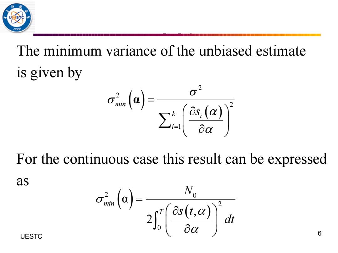
/9 The minimum variance of the unbiased estimate is given by For the continuous case this result can be expressed as N dt UESTC 6
The minimum variance of the unbiased estimate is given by For the continuous case this result can be expressed as 6 UESTC ( ) ( ) 2 2 2 1 min k i i s = = α ( ) ( ) 2 0 2 0 α , 2 min T N s t dt =

11.4 Amplitude estimation in the coherent case with WGN Assume the phase is known and the amplitude must be estimated. y;=aS+n,i=1,.,k The amplitude a can either be a random variable of an unknown constant. ML: -a四-0+2(0ag0 i=l Symbol energy UESTC ∑y e=∑s 7 i=l
11.4 Amplitude estimation in the coherent case with WGN Assume the phase is known and the amplitude must be estimated. The amplitude a can either be a random variable of an unknown constant. ML: 7 UESTC , 1, , i i i y n = + = as i k ( ( )) ( ) 1 0 k i i i i s y s = − = ( ) 1 0 k i i i i as s = y − = 1 1 k ML i i i a s = = y ε 2 1 k i i s = ε= Symbol energy

The mean of this estimate is Ea=a,it is unbiased.The variance of it is .According to we have o≥o2/e It can be seen that the estimate is efficient. A MAP estimate can be obtained by selecting an a priori distribution of p(a). UESTC 8
The mean of this estimate is , it is unbiased. The variance of it is . According to we have It can be seen that the estimate is efficient. A MAP estimate can be obtained by selecting an a priori distribution of . 8 UESTC E a aML = 2 ε ( ) ( ) 2 2 2 1 min k i i s = = α 2 2 aˆ ε p a( )
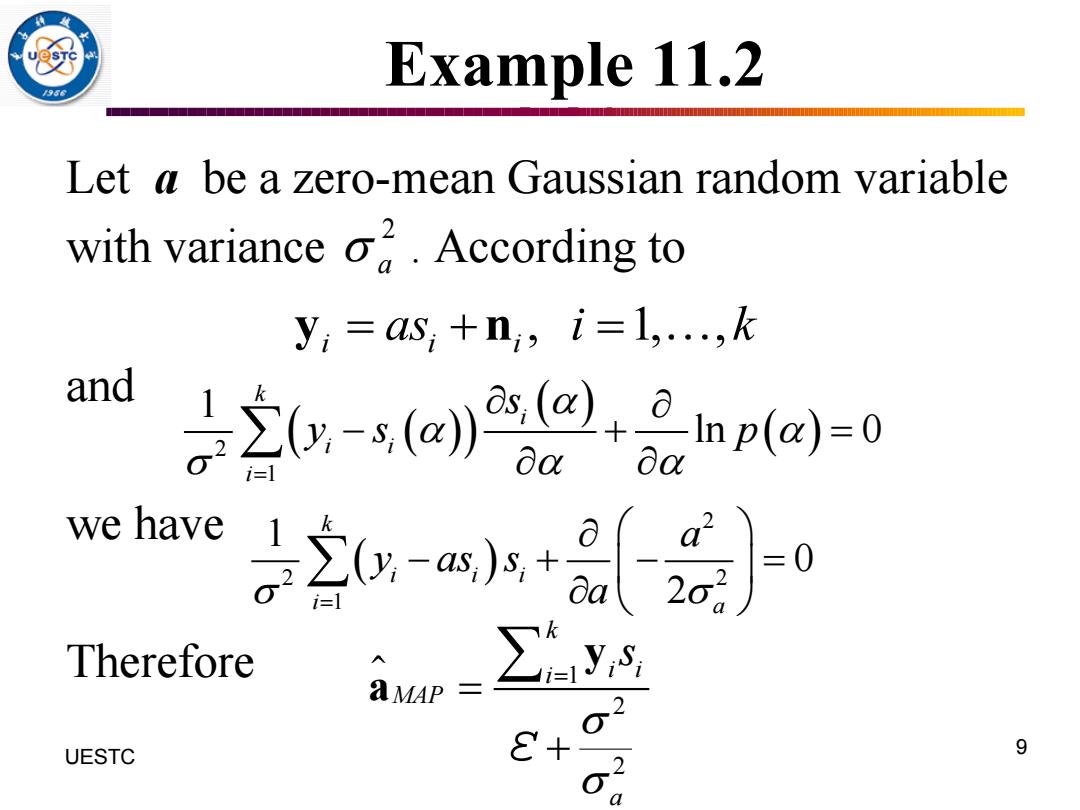
Example 11.2 Let a be a zero-mean Gaussian random variable with varianceo.According to y:=aS,+n,i=1,…,k and 空to但ana-0 aa we have 合0w+}-0 Therefore ∑y aMAP 2 UESTC E+ 9 2
Example 11.2 Let a be a zero-mean Gaussian random variable with variance . According to and we have Therefore 9 UESTC 2 a , 1, , i i i y n = + = as i k ( ( )) ( ) ( ) 2 1 1 ln 0 k i i i i s y s p = − + = ( ) 2 2 2 1 1 0 2 k i i i i a a y as s = a − + − = 1 2 2 k i i i MAP a s = = + y a ε
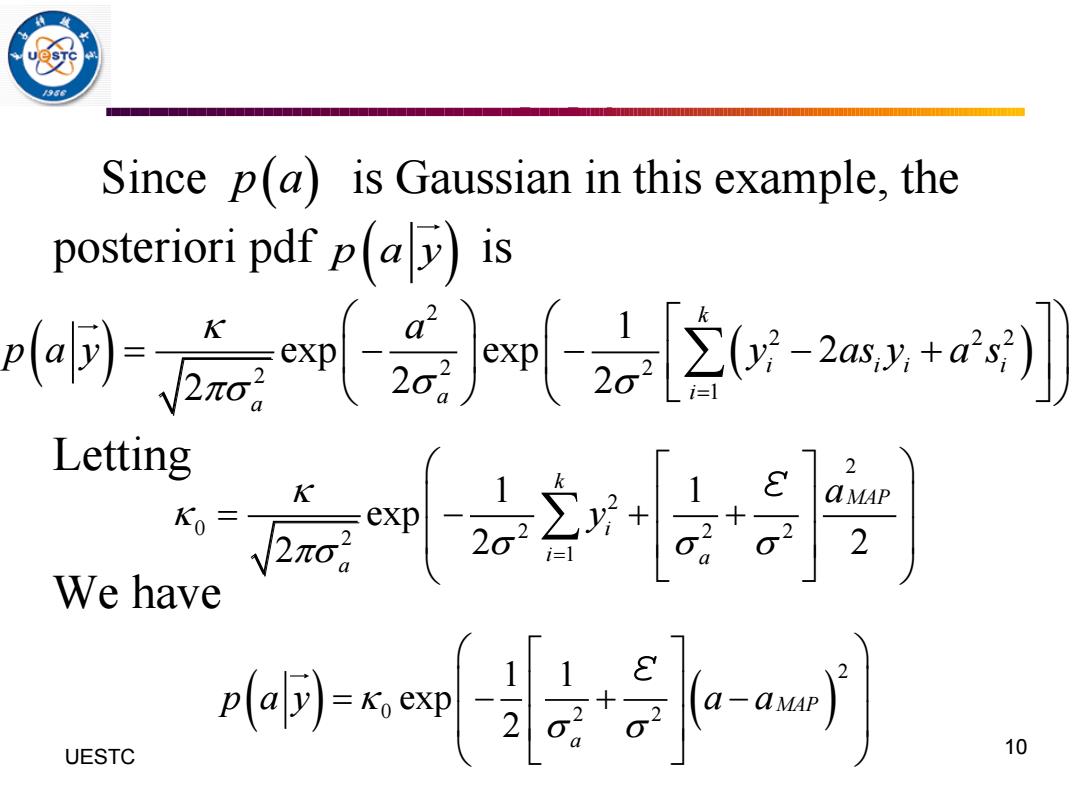
Since p(a)is Gaussian in this example,the posteriori pdf p(is 点m最-ar+刘 Letting 2 K We have UESTC 10
Since is Gaussian in this example, the posteriori pdf is Letting We have 10 UESTC p a( ) p a y ( ) ( ) ( ) 2 2 2 2 2 2 2 1 1 exp exp 2 2 2 2 k i i i i a i a a p a y y as y a s = = − − − + 2 2 0 2 2 2 2 1 1 1 exp 2 2 2 k MAP i i a a a y = = − + + ε ( ) ( ) 2 0 2 2 1 1 exp 2 MAP a p a y a a = − + − ε