Gradient descent
Gradient Descent

Review:Gradient Descent In step 3,we have to solve the following optimization problem: θ*=arg min L(0) L:loss functionθ:parameters Suppose that 0 has two variables {01,02} Randomly start at 00 09] 7L(0)= 0L(01)/a61 1aL(02)/a02 [aL(0)/a61 02 aL(0)/a62 01=00-nL(0) aL(0)/a61 aL(02)/a02 → 02=01-n7L(01)
Review: Gradient Descent • In step 3, we have to solve the following optimization problem: 𝜃 ∗ = arg min 𝜃 𝐿 𝜃 L: loss function 𝜃: parameters Suppose that θ has two variables {θ1 , θ2 } Randomly start at 𝜃 0 = 𝜃1 0 𝜃2 0 𝛻𝐿 𝜃 = 𝜕𝐿 𝜃1 Τ𝜕𝜃1 𝜕𝐿 𝜃2 Τ𝜕𝜃2 𝜃1 1 𝜃2 1 = 𝜃1 0 𝜃2 0 − 𝜂 𝜕𝐿 𝜃1 Τ 0 𝜕𝜃1 𝜕𝐿 𝜃2 Τ 0 𝜕𝜃2 𝜃 1 = 𝜃 0 − 𝜂𝛻𝐿 𝜃 0 𝜃1 2 𝜃2 2 = 𝜃1 1 𝜃2 1 − 𝜂 𝜕𝐿 𝜃1 Τ 1 𝜕𝜃1 𝜕𝐿 𝜃2 Τ 1 𝜕𝜃2 𝜃 2 = 𝜃 1 − 𝜂𝛻𝐿 𝜃 1
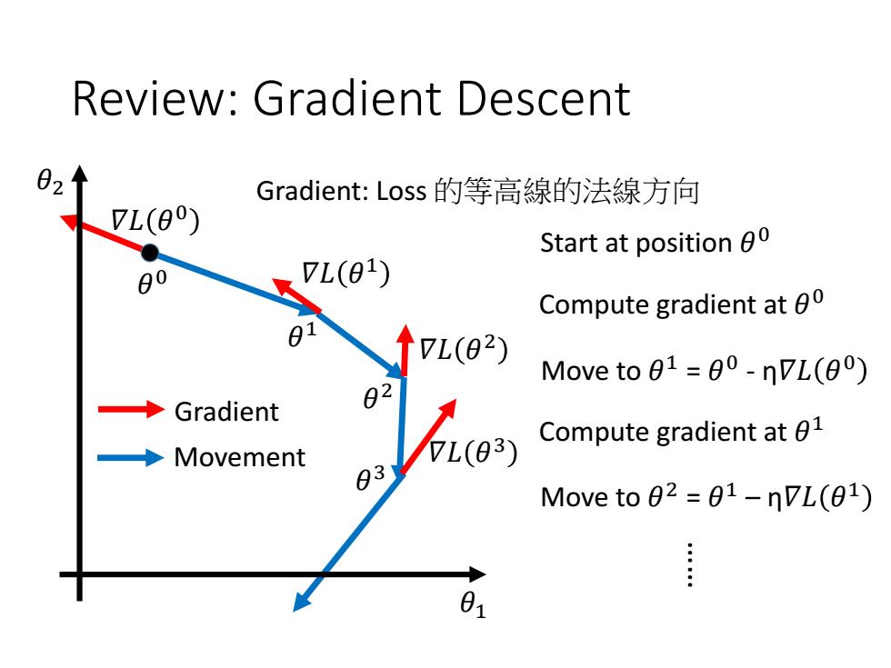
Review:Gradient Descent Gradient:Loss的等高線的法線方向 L(0) Start at position 00 80 7L(01) Compute gradient at 0 7L(02) Move to 01=00-nVL(00) ◆ Gradient 82 Movement L(03) Compute gradient at 01 83 Move to 02 =01-nVL(01) 01
Review: Gradient Descent Start at position 𝜃 0 Compute gradient at 𝜃 0 Move to 𝜃 1 = 𝜃 0 - η𝛻𝐿 𝜃 0 Compute gradient at 𝜃 1 Move to 𝜃 2 = 𝜃 1 – η𝛻𝐿 𝜃 1 Movement Gradient …… 𝜃 0 𝜃 1 𝜃 2 𝜃 3 𝛻𝐿 𝜃 0 𝛻𝐿 𝜃 1 𝛻𝐿 𝜃 2 𝛻𝐿 𝜃 3 𝜃1 𝜃2 Gradient: Loss 的等高線的法線方向
Gradient descent Tip 1:Tuning your learning rates
Gradient Descent Tip 1: Tuning your learning rates
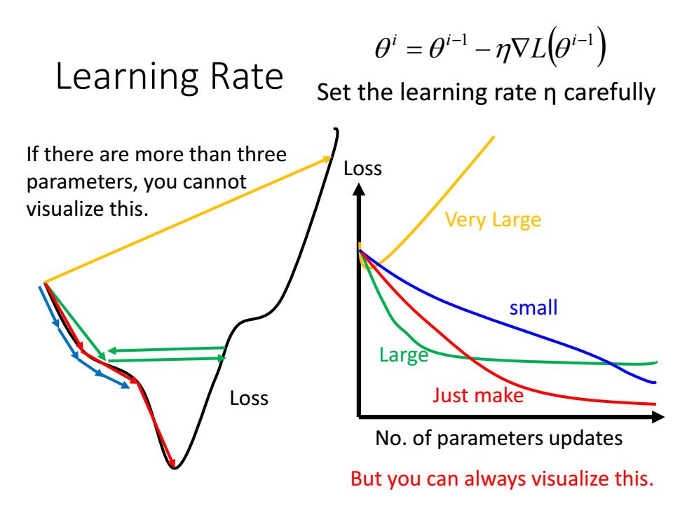
0=0-1-VL0-1) Learning Rate Set the learning rate n carefully If there are more than three Loss parameters,you cannot visualize this. Very Large small Large Loss Just make No.of parameters updates But you can always visualize this
Learning Rate No. of parameters updates Loss Loss Very Large Large small Just make 1 1 i i i L Set the learning rate η carefully If there are more than three parameters, you cannot visualize this. But you can always visualize this
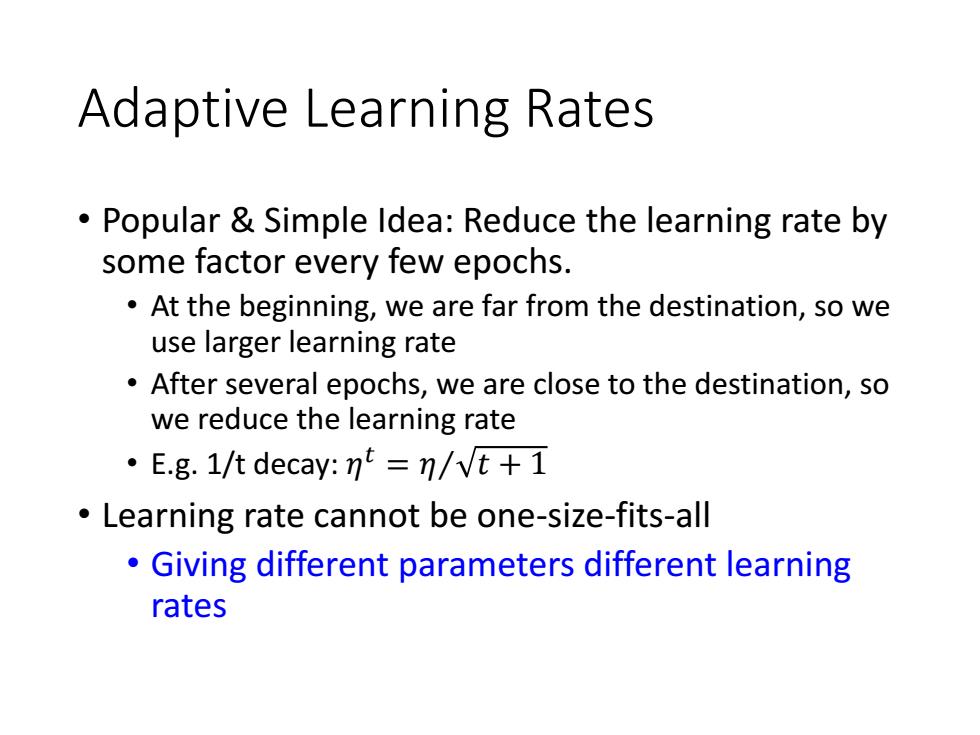
Adaptive Learning Rates Popular Simple Idea:Reduce the learning rate by some factor every few epochs. At the beginning,we are far from the destination,so we use larger learning rate After several epochs,we are close to the destination,so we reduce the learning rate E.g.1/t decay:n=n/vt+1 Learning rate cannot be one-size-fits-all Giving different parameters different learning rates
Adaptive Learning Rates • Popular & Simple Idea: Reduce the learning rate by some factor every few epochs. • At the beginning, we are far from the destination, so we use larger learning rate • After several epochs, we are close to the destination, so we reduce the learning rate • E.g. 1/t decay: 𝜂 𝑡 = 𝜂Τ 𝑡 + 1 • Learning rate cannot be one-size-fits-all • Giving different parameters different learning rates
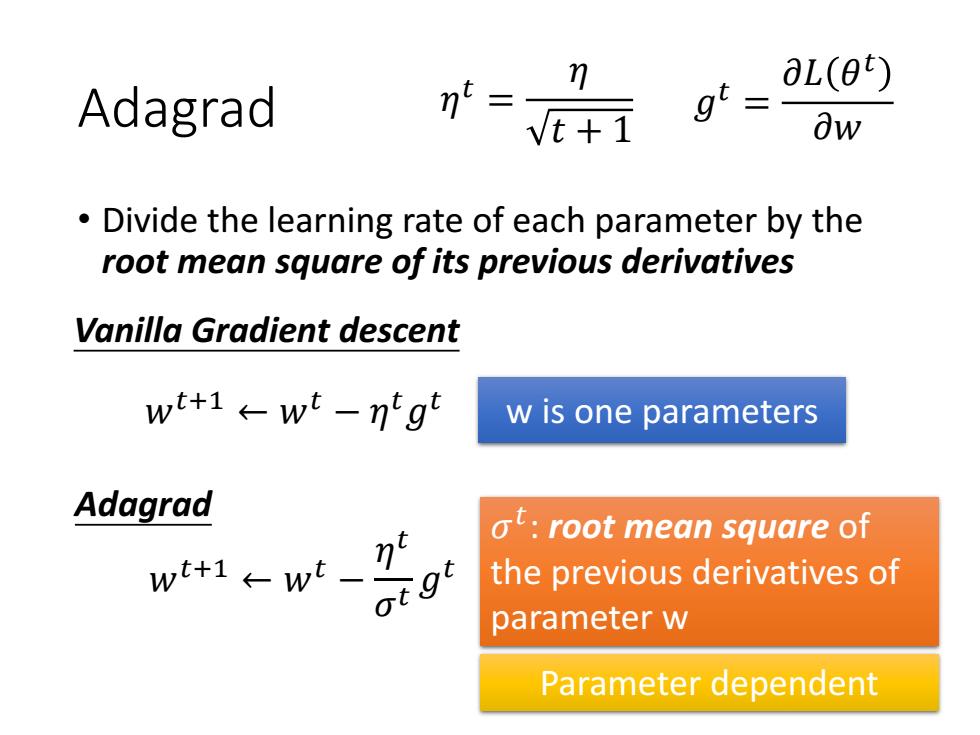
aL(0) Adagrad nt vt+1 gt 0w Divide the learning rate of each parameter by the root mean square of its previous derivatives Vanilla Gradient descent wt+1←wt-ng w is one parameters Adagrad ot:root mean square of w+1←wt_刀 the previous derivatives of parameter w Parameter dependent
Adagrad • Divide the learning rate of each parameter by the root mean square of its previous derivatives 𝜎 𝑡 : root mean square of the previous derivatives of parameter w w is one parameters 𝑔 𝑡 = 𝜕𝐿 𝜃 𝑡 𝜕𝑤 Vanilla Gradient descent Adagrad 𝑤𝑡+1 ← 𝑤𝑡 − 𝜂 𝑡𝑔 𝑡 𝜂 𝑡 = 𝜂 𝑡 + 1 𝑤𝑡+1 ← 𝑤𝑡 − 𝜂 𝑡 𝜎 𝑡 𝑔 𝑡 Parameter dependent
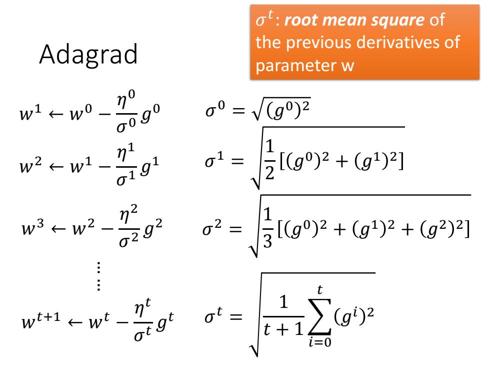
ot:root mean square of the previous derivatives of Adagrad parameter w w1←w0一 o090 0=V(g)2 w2←w1- 91 01=【g2+g鬥 w3←w22 0292 2-层g92+g+g1 w+1←wt-刀 1 t+ g)2 0
Adagrad 𝑤1 ← 𝑤0 − 𝜂 0 𝜎 0 𝑔 0 … … 𝑤2 ← 𝑤1 − 𝜂 1 𝜎 1 𝑔 1 𝑤𝑡+1 ← 𝑤𝑡 − 𝜂 𝑡 𝜎 𝑡 𝑔 𝑡 𝜎 0 = 𝑔0 2 𝜎 1 = 1 2 𝑔0 2 + 𝑔1 2 𝜎 𝑡 = 1 𝑡 + 1 𝑖=0 𝑡 𝑔𝑖 2 𝑤3 ← 𝑤2 − 𝜂 2 𝜎 2 𝑔 2 𝜎 2 = 1 3 𝑔0 2 + 𝑔1 2 + 𝑔2 2 𝜎 𝑡 : root mean square of the previous derivatives of parameter w
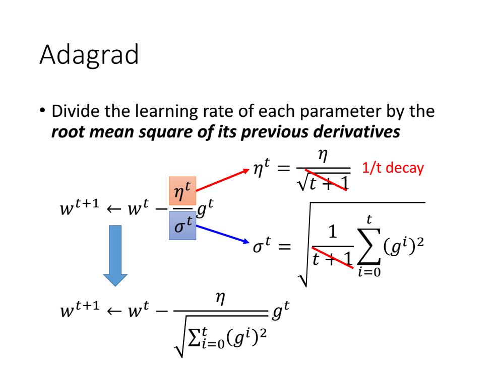
Adagrad Divide the learning rate of each parameter by the root mean square of its previous derivatives n-vt+i 1/t decay wt+1←wt wt+1←wt ∑=o(g)2
Adagrad • Divide the learning rate of each parameter by the root mean square of its previous derivatives 𝜂 𝑡 = 𝜂 𝑡 + 1 𝑤𝑡+1 ← 𝑤𝑡 − 𝜂 σ𝑖=0 𝑡 𝑔𝑖 2 𝑔 𝑡 1/t decay 𝑤𝑡+1 ← 𝑤𝑡 − 𝜂 𝜎 𝑡 𝑔 𝑡 𝜎 𝑡 = 1 𝑡 + 1 𝑖=0 𝑡 𝑔𝑖 2 𝜂 𝑡 𝜎 𝑡

Contradiction?-=vz gi= aL(0t) 0w Vanilla Gradient descent w+1←wt-ng Larger gradient, larger step Adagrad Larger gradient, w+1←wt、 larger step =9 (g2 Larger gradient, smaller step
Contradiction? 𝑤𝑡+1 ← 𝑤𝑡 − 𝜂 σ𝑖=0 𝑡 𝑔𝑖 2 𝑔 𝑡 Vanilla Gradient descent Adagrad Larger gradient, larger step Larger gradient, smaller step Larger gradient, larger step 𝑤𝑡+1 ← 𝑤𝑡 − 𝜂 𝑡𝑔 𝑡 𝑔 𝑡 = 𝜕𝐿 𝜃 𝑡 𝜕𝑤 𝜂 𝑡 = 𝜂 𝑡 + 1