Chapter 2 Linear Regression
Chapter 2 Linear Regression

Contents 。2.1 Introduction 2.2 Polynomial Curve Fitting:A Toy 。2.3Over-fitting 2.4 Cross-Validation ·2.5 Regularization 2.6 Linear Basis Function Models 2.7 Least Squares Revisited 2.8 Bayesian Linear Regression
Contents • 2.1 Introduction • 2.2 Polynomial Curve Fitting: A Toy • 2.3 Over-fitting • 2.4 Cross-Validation • 2.5 Regularization • 2.6 Linear Basis Function Models • 2.7 Least Squares Revisited • 2.8 Bayesian Linear Regression
2.1 Introduction Supervised learning:regression and classification.The goal of regression is to predict the value of one or more continuous target variable given the value of a p-dimensional vector of input variables. In linear regression,the model for such a relationship is a linear model. Alinear regression example:given a ata set linear regression model assumes that the relationship between the target variable yi and the p-dimensional vector of input variables xi is linear,i.e. yi=Bixu++Bpxip +s=xB+ i=1,.,n
2.1 Introduction • Supervised learning: regression and classification. The goal of regression is to predict the value of one or more continuous target variable given the value of a p-dimensional vector of input variables. • In linear regression, the model for such a relationship is a linear model. • A linear regression example: given a data set , a linear regression model assumes that the relationship between the target variable and the p-dimensional vector of input variables is linear, i.e
2.1.1 History for Regression The earliest form of regression was the method of least squares,which was published by Legendre in 1805,and by Gauss in 1809. ·The term"regression(倒退,退步)"was coined by Francis Galton in the 19th century to describe Gauss Francis Galton a biological phenomenon.The phenomenon was that the heights of descendants of tall ancestors tend to regress down towards a normal average. Galton's work was later extended by Udny Yule and Karl Pearson to a more general statistical context. Udny Yule Karl Pearson
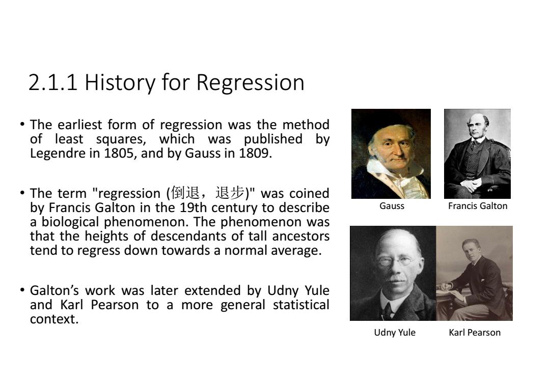
2.1.1 History for Regression • The earliest form of regression was the method of least squares, which was published by Legendre in 1805, and by Gauss in 1809. • The term "regression (倒退,退步)" was coined by Francis Galton in the 19th century to describe a biological phenomenon. The phenomenon was that the heights of descendants of tall ancestors tend to regress down towards a normal average. • Galton’s work was later extended by Udny Yule and Karl Pearson to a more general statistical context. Gauss Francis Galton Udny Yule Karl Pearson
2.1.2 Development for Regression Regression methods continue to be an active research area. New methods have been developed for √robust regression regression involving correlated responses such as time series and growth curves regression in which the predictor (independent variable)or response variables are curves, images,graphs,or other complex data objects regression methods accommodating various types of missing data,nonparametric regression Bayesian methods for regression regression in which the predictor variables are measured with error regression with more predictor variables than observations causal inference with regression
2.1.2 Development for Regression • Regression methods continue to be an active research area . • New methods have been developed for robust regression regression involving correlated responses such as time series and growth curves regression in which the predictor (independent variable) or response variables are curves, images, graphs, or other complex data objects regression methods accommodating various types of missing data, nonparametric regression Bayesian methods for regression regression in which the predictor variables are measured with error regression with more predictor variables than observations causal inference with regression
2.2 Polynomial Curve Fitting:A Toy Suppose we have a training set ti,,from xN+1,we want to predict tN+1. In this certain case,the training set is generated from t=f(x)=sin(2πx) 。 Green curve is the original function and the blue circles are noise polluted samples.Here N =10. The goal for regression is to predict the value of t for some new value of x without knowledge of the green curve
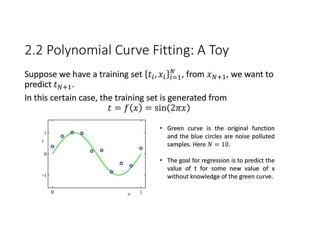
2.2 Polynomial Curve Fitting: A Toy Suppose we have a training set , from , we want to predict . In this certain case, the training set is generated from • Green curve is the original function and the blue circles are noise polluted samples. Here . • The goal for regression is to predict the value of t for some new value of x without knowledge of the green curve
2.2 Polynomial Curve Fitting:A Toy The prediction objective is intrinsically difficult in that we have to generalize from a finite and noise-corrupted data set. We have many approaches to deal with this regression,here for our teaching purpose,we adopt this linear polynomial model. ·Suppose,f(x,W)=w0+ω1x+ω2x2+..+WMxM where M is the order of the polynomial
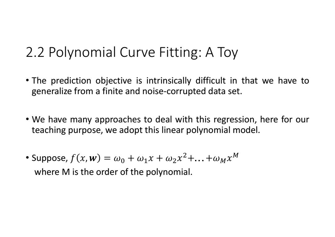
2.2 Polynomial Curve Fitting: A Toy • The prediction objective is intrinsically difficult in that we have to generalize from a finite and noise-corrupted data set. • We have many approaches to deal with this regression, here for our teaching purpose, we adopt this linear polynomial model. • Suppose, where M is the order of the polynomial
2.2 Polynomial Curve Fitting:A Toy The values of the coefficients will be determined by fitting the polynomial to the training data. To do this,we can minimize an error function which measures the misfit between f(x,w)and the training set w.r.t w. A natural choice of error function is E0w)=2∑fw)-tn m=
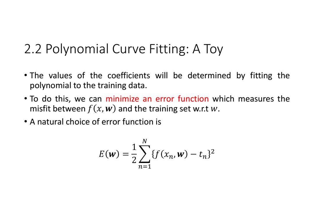
2.2 Polynomial Curve Fitting: A Toy • The values of the coefficients will be determined by fitting the polynomial to the training data. • To do this, we can minimize an error function which measures the misfit between and the training set w.r.t . • A natural choice of error function is
2.2 Polynomial Curve Fitting:A Toy ·E(w)=2∑m1f(x,wW)-tn2=2∑m=1{x7w-tn2 where xn [1 xnx...xM] Further simplifications yield E(w)=2∑wrxw-2tw+ n=1 Setting the derivative of E(w)equal to 0,we have: ∑xnw=∑tnxn n=1 n=1 By solving this equation,we get the optimum w in least square sense
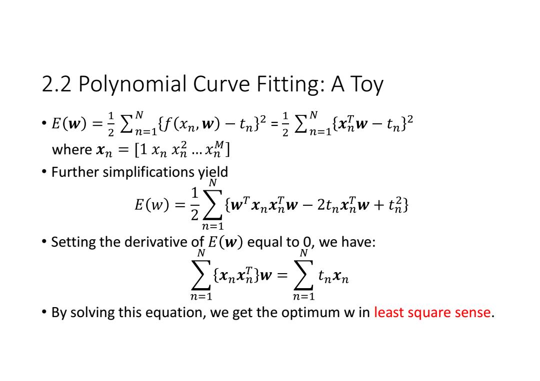
2.2 Polynomial Curve Fitting: A Toy • = where • Further simplifications yield • Setting the derivative of equal to 0, we have: • By solving this equation, we get the optimum w in least square sense
2.2 Polynomial Curve Fitting:A Toy The first question is:does the above equation have a solution??? Put the question aside for now,let's see the fitting result.Here we assume we have 10 training samples,i.e.N=10. Oth Order Polynomial 1st Order Polynomial M=0 M=1 0 0
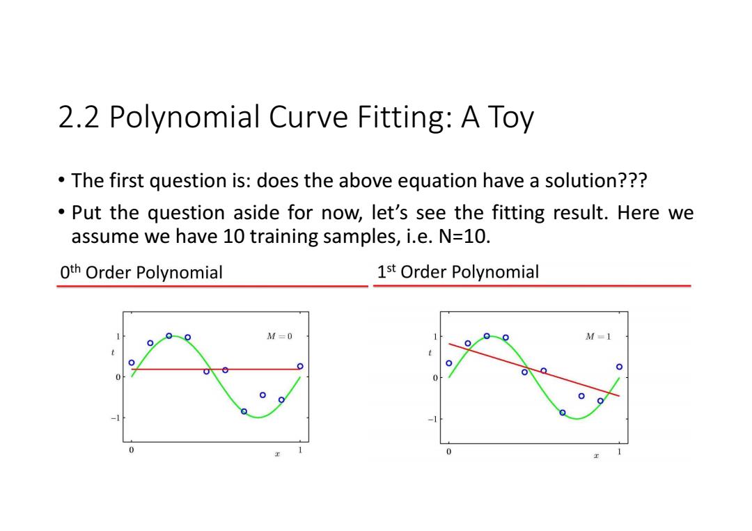
2.2 Polynomial Curve Fitting: A Toy • The first question is: does the above equation have a solution??? • Put the question aside for now, let’s see the fitting result. Here we assume we have 10 training samples, i.e. N=10