Journal of Monetary Economics 15(1985)145-161.North-Holland THE EQUITY PREMIUM A Puzzle* Rajnish MEHRA Columbia University,New York,NY 10027,USA Edward C.PRESCOTT Federal Reserve Bank of Minneapolis University of Minnesota,Minneapolis,MN 55455,USA. Restrictions that a class of general equilibrium models place upon the average returns of equity and Treasury bills are found to be strongly violated by the U.S.data in the 1889-1978 period.This result is robust to model specification and measurement problems.We conclude that,most likely, an equilibrium model which is not an Arrow-Debreu economy will be the one that simultaneously rationalizes both historically observed large average equity return and the small average risk-free return. 1.Introduction Historically the average return on equity has far exceeded the average return on short-term virtually default-free debt.Over the ninety-year period 1889-1978 the average real annual yield on the Standard and Poor 500 Index was seven percent,while the average yield on short-term debt was less than one percent. The question addressed in this paper is whether this large differential in average yields can be accounted for by models that abstract from transactions costs,liquidity constraints and other frictions absent in the Arrow-Debreu set-up.Our finding is that it cannot be,at least not for the class of economies considered.Our conclusion is that most likely some equilibrium model with a *This research was initiated at the University of Chicago where Mehra was a visiting scholar at the Graduate School of Business and Prescott a Ford foundation visiting professor at the Department of Economics.Earlier versions of this paper,entitled 'A Test of the Intertemporal Asset Pricing Model',were presented at the University of Minnesota,University of Lausanne, Harvard University,NBER Conference on Intertemporal Puzzles in Macroeconomics,and the American Finance Meetings.We wish to thank the workshop participants,George Constantinides, Eugene Fama,Merton Miller,and particularly an anonymous referee,Fischer Black,Stephen LeRoy and Charles Plosser for helpful discussions and constructive criticisms.We gratefully acknowledge financial support from the Faculty Research Fund of the Graduate School of Business,Columbia University,the National Science Foundation and the Federal Reserve Bank of Minneapolis. 0304-3923/85/$3.301985,Elsevier Science Publishers B.V.(North-Holland)

146 R.Mehra and E.C.Prescott,The equity premium friction will be the one that successfully accounts for the large average equity premium. We study a class of competitive pure exchange economies for which the equilibrium growth rate process on consumption and equilibrium asset returns are stationary.Attention is restricted to economies for which the elasticity of substitution for the composite consumption good between the year t and year t+1 is consistent with findings in micro,macro and international economics. In addition,the economies are constructed to display equilibrium consumption growth rates with the same mean,variance and serial correlation as those observed for the U.S.economy in the 1889-1978 period.We find that for such economies,the average real annual yield on equity is a maximum of four-tenths of a percent higher than that on short-term debt,in sharp contrast to the six percent premium observed.Our results are robust to non-stationarities in the means and variances of the economies'growth processes. The simple class of economies studied,we think,is well suited for the question posed.It clearly is poorly suited for other issues,in particular issues such as the volatility of asset prices.We emphasize that our analysis is not an estimation exercise,which is designed to obtain better estimates of key economic parameters.Rather it is a quantitative theoretical exercise designed to address a very particular question.2 Intuitively,the reason why the low average real return and high average return on equity cannot simultaneously be rationalized in a perfect market framework is as follows:With real per capita consumption growing at nearly two percent per year on average,the elasticities of substitution between the year t and year t+1 consumption good that are sufficiently small to yield the six percent average equity premium also yield real rates of return far in excess of those observed.In the case of a growing economy,agents with high risk aversion effectively discount the future to a greater extent than agents with low risk aversion (relative to a non-growing economy).Due to growth,future consumption will probably exceed present consumption and since the marginal utility of future consumption is less than that of present consumption,real interest rates will be higher on average. This paper is organized as follows:Section 2 summarizes the U.S.historical experience for the ninety-year period 1889-1978.Section 3 specifies the set of economies studied.Their behavior with respect to average equity and short-term debt yields,as well as a summary of the sensitivity of our results to the specifications of the economy,are reported in section 4.Section 5 concludes the paper. 1There are other interesting features of time series and procedures for testing them.The variance bound tests of LeRoy and Porter (1981)and Shiller (1980)are particularly innovative and constructive.They did indicate that consumption risk was important [see Grossman and Shiller (1981)and LeRoy and LaCavita(1981)]. 2See Lucas(1980)for an articulation of this methodology
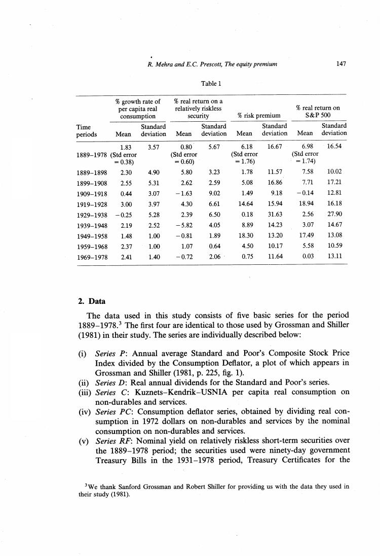
R.Mehra and E.C.Prescott,The equity premium 147 Table 1 %growth rate of real return on a per capita real relatively riskless real return on consumption security %risk premium S&P500 Time Standard Standard Standard Standard periods Mean deviation Mean deviation Mean deviation Mean deviation 1.83 3.57 0.80 5.67 6.18 16.67 6.98 16.54 1889-1978 (Std error (Std error (Std error (Std error =0.38) =0.60) =1.76) =1.74) 1889-1898 2.30 4.90 5.80 3.23 1.78 11.57 7.58 10.02 1899-1908 2.55 5.31 2.62 2.59 5.08 16.86 7.71 17.21 1909-1918 0.44 3.07 -1.63 9.02 1.49 9.18 -0.14 12.81 1919-1928 3.00 3.97 4.30 6.61 14.64 15.94 18.94 16.18 1929-1938 -0.25 5.28 2.39 6.50 0.18 31.63 2.56 27.90 1939-1948 2.19 2.52 -5.82 4.05 8.89 14.23 3.07 14.67 1949-1958 1.48 1.00 -0.81 1.89 18.30 13.20 17.49 13.08 1959-1968 2.37 1.00 1.07 0.64 4.50 10.17 5.58 10.59 1969-1978 2.41 1.40 -0.72 2.06 0.75 11.64 0.03 13.11 2.Data The data used in this study consists of five basic series for the period 1889-1978.3 The first four are identical to those used by Grossman and Shiller (1981)in their study.The series are individually described below: (i)Series P:Annual average Standard and Poor's Composite Stock Price Index divided by the Consumption Deflator,a plot of which appears in Grossman and Shiller(1981,p.225,fig.1). (ii)Series D:Real annual dividends for the Standard and Poor's series. (ii)Series C:Kuznets-Kendrik-USNIA per capita real consumption on non-durables and services. (iv)Series PC:Consumption deflator series,obtained by dividing real con- sumption in 1972 dollars on non-durables and services by the nominal consumption on non-durables and services. (v)Series RF:Nominal yield on relatively riskless short-term securities over the 1889-1978 period;the securities used were ninety-day government Treasury Bills in the 1931-1978 period,Treasury Certificates for the 3We thank Sanford Grossman and Robert Shiller for providing us with the data they used in their study (1981)
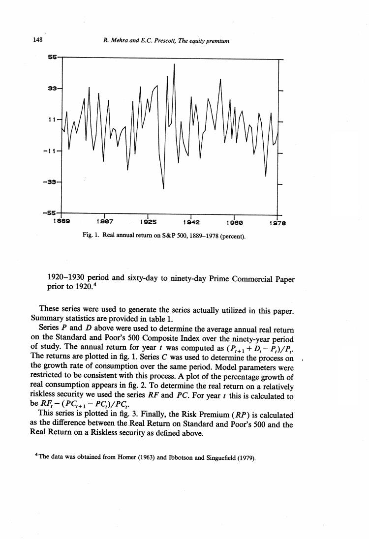
148 R.Mehra and E.C.Prescott,The equity premium -33 -55- 1889 19e7 1925 1942 1980 1978 Fig.1.Real annual return on S&P 500,1889-1978(percent). 1920-1930 period and sixty-day to ninety-day Prime Commercial Paper prior to 1920.4 These series were used to generate the series actually utilized in this paper. Summary statistics are provided in table 1. Series P and D above were used to determine the average annual real return on the Standard and Poor's 500 Composite Index over the ninety-year period of study.The annual return for year t was computed as (P++D,-P,)/P The returns are plotted in fig.1.Series C was used to determine the process on the growth rate of consumption over the same period.Model parameters were restricted to be consistent with this process.A plot of the percentage growth of real consumption appears in fig.2.To determine the real return on a relatively riskless security we used the series RF and PC.For year t this is calculated to be RF:-(PC:+1-PC,)/PC This series is plotted in fig.3.Finally,the Risk Premium(RP)is calculated as the difference between the Real Return on Standard and Poor's 500 and the Real Return on a Riskless security as defined above. 4The data was obtained from Homer(1963)and Ibbotson and Singuefield(1979)
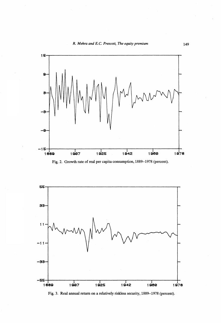
R.Mehra and E.C.Prescott,The equity premium 149 15 9 -15 1889 1907 1925 1942 1960 1878 Fig.2.Growth rate of real per capita consumption,1889-1978(percent). 55 -33 -55- 1889 1987 1925 1942 196e 1978 Fig.3.Real annual return on a relatively riskless security,1889-1978(percent)

150 R.Mehra and E.C.Prescott,The equity premium 3.The economy,asset prices and returns In this paper,we employ a variation of Lucas'(1978)pure exchange model. Since per capita consumption has grown over time,we assume that the growth rate of the endowment follows a Markov process.This is in contrast to the assumption in Lucas'model that the endowment level follows a Markov process.Our assumption,which requires an extension of competitive equi- librium theory,enables us to capture the non-stationarity in the consumption series associated with the large increase in per capita consumption that occurred in the 1889-1978 period. The economy we consider was judiciously selected so that the joint process governing the growth rates in aggregate per capita consumption and asset prices would be stationary and easily determined.The economy has a single representative'stand-in'household.This unit orders its preferences over ran- dom consumption paths by e 0<B<1, (1) where c,is per capita consumption,B is the subjective time discount factor, Eof}is the expectation operator conditional upon information available at time zero (which denotes the present time)and U:RR is the increasing concave utility function.To insure that the equilibrium return process is stationary,the utility function is further restricted to be of the constant relative risk aversion class, U(c,a)=c--1 1-a3 0<a<0 (2) The parameter a measures the curvature of the utility function.When a is equal to one,the utility function is defined to be the logarithmic function, which is the limit of the above function as a approaches one. We assume that there is one productive unit producing the perishable consumption good and there is one equity share that is competitively traded. Since only one productive unit is considered,the return on this share of equity is also the return on the market.The firm's output is constrained to be less than or equal to y.It is the firm's dividend payment in the period t as well. The growth rate in y,is subject to a Markov chain;that is, y+1=X+1乃, (3)
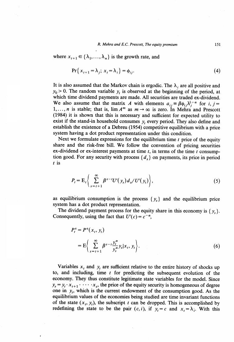
R.Mehra and E.C.Prescott,The equity premium 151 where x,.+1∈{入l,,入n}is the growth rate,.and Pr{x+1=入yix,=入}=中 (4) It is also assumed that the Markov chain is ergodic.The A,are all positive and yo>0.The random variable y,is observed at the beginning of the period,at which time dividend payments are made.All securities are traded ex-dividend. We also assume that the matrix A with elements a=for i,j= 1,...,n is stable;that is,lim A"as moo is zero.In Mehra and Prescott (1984)it is shown that this is necessary and sufficient for expected utility to exist if the stand-in household consumes y,every period.They also define and establish the existence of a Debreu(1954)competitive equilibrium with a price system having a dot product representation under this condition. Next we formulate expressions for the equilibrium time t price of the equity share and the risk-free bill.We follow the convention of pricing securities ex-dividend or ex-interest payments at time t,in terms of the time t consump- tion good.For any security with process {d}on payments,its price in period t is P=E,2g-U)da,/}: (5) =1+1 as equilibrium consumption is the process {y,and the equilibrium price system has a dot product representation. The dividend payment process for the equity share in this economy is {y,) Consequently,using the fact that U'(c)=c-, pe=pe(x,y (6) s=t+1 Variables x,and y,are sufficient relative to the entire history of shocks up to,and including,time t for predicting the subsequent evolution of the economy.They thus constitute legitimate state variables for the model.Since y,=y,'xz+l··,··xs,the price of the equity security is homogeneous of degree one in y,which is the current endowment of the consumption good.As the equilibrium values of the economies being studied are time invariant functions of the state (xy),the subscript t can be dropped.This is accomplished by redefining the state to be the pair (c,i),if y=c and x,=Ai.With this
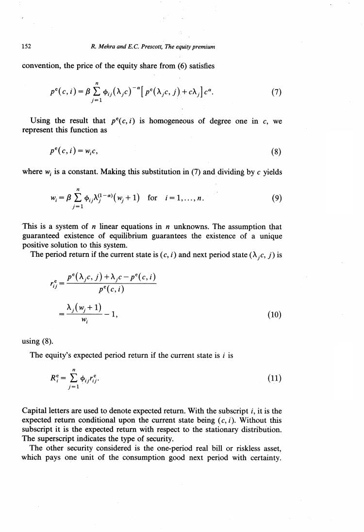
152 R.Mehra and E.C.Prescott,The equity premium convention,the price of the equity share from(6)satisfies p(c,i)=B∑中,(c)[p(c,)+cc (7) Using the result that pe(c,i)is homogeneous of degree one in c,we represent this function as pe(c,i)=wc, (8) where w is a constant.Making this substitution in(7)and dividing by c yields w=Bw+1)for i=1.....n. (9) =1 This is a system of n linear equations in n unknowns.The assumption that guaranteed existence of equilibrium guarantees the existence of a unique positive solution to this system. The period return if the current state is(c,i)and next period state(A c,j)is 方-pas功+Ac-pc,) pe(c,i) 入(%+1) (10) 州 1, using (8). The equity's expected period return if the current state is i is R=∑ (11) i=1 Capital letters are used to denote expected return.With the subscript i,it is the expected return conditional upon the current state being (c,i).Without this subscript it is the expected return with respect to the stationary distribution. The superscript indicates the type of security. The other security considered is the one-period real bill or riskless asset, which pays one unit of the consumption good next period with certainty
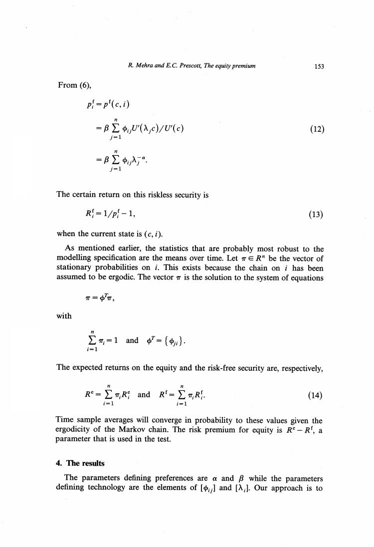
R.Mehra and E.C.Prescott,The equity premium 153 From (6), p=p'(c,i) =BΣ中U(入c)/U(c) (12) j=1 =B∑中入 =1 The certain return on this riskless security is R=1/p-1, (13) when the current state is (c,i). As mentioned earlier,the statistics that are probably most robust to the modelling specification are the means over time.Let TER"be the vector of stationary probabilities on i.This exists because the chain on i has been assumed to be ergodic.The vector is the solution to the system of equations π=Tπ, with 1and ={$} i-1 The expected returns on the equity and the risk-free security are,respectively, Re-∑m,R and Rf-∑m,R. (14) =1 Time sample averages will converge in probability to these values given the ergodicity of the Markov chain.The risk premium for equity is Re-R,a parameter that is used in the test. 4.The results The parameters defining preferences are a and B while the parameters defining technology are the elements of [and [A,].Our approach is to

154 R.Mehra and E.C.Prescott,The equity premium assume two states for the Markov chain and to restrict the process as follows: 入1=1+4+6,入2=1+4-8, φ11=中22=中, φ12=中21=(1-中) The parameters u,,and 6 now define the technology.We require 8>0 and 0<<1.This particular parameterization was selected because it permitted us to independently vary the average growth rate of output by changing u,the variability of consumption by altering 6,and the serial correlation of growth rates by adjustingφ. The parameters were selected so that the average growth rate of per capita consumption,the standard deviation of the growth rate of per capita consump- tion and the first-order serial correlation of this growth rate,all with respect to the model's stationary distribution,matched the sample values for the U.S. economy between 1889-1978.The sample values for the U.S.economy were 0.018,0.036 and -0.14,respectively.The resulting parameter's values were u=0.018,8=0.036 and =0.43.Given these values,the nature of the test is to search for parameters a and B for which the model's averaged risk-free rate and equity risk premium match those observed for the U.S.economy over this ninety-year period. The parameter a,which measures peoples'willingness to substitute con- sumption between successive yearly time periods is an important one in many fields of economics.Arrow (1971)summarizes a number of studies and concludes that relative risk aversion with respect to wealth is almost constant. He further argues on theoretical grounds that a should be approximately one. Friend and Blume (1975)present evidence based upon the portfolio holdings of individuals that a is larger,with their estimates being in the range of two. Kydland and Prescott (1982),in their study of aggregate fluctuations,found that they needed a value between one and two to mimic the observed relative variabilities of consumption and investment.Altug (1983),using a closely related model and formal econometric techniques,estimates the parameter to be near zero.Kehoe (1984),studying the response of small countries balance of trade to terms of trade shocks,obtained estimates near one,the value posited by Arrow.Hildreth and Knowles (1982)in their study of the behavior of farmers also obtain estimates between one and two.Tobin and Dolde (1971), studying life cycle savings behavior with borrowing constraints,use a value of 1.5 to fit the observed life cycle savings patterns. Any of the above cited studies can be challenged on a number of grounds but together they constitute an a priori justification for restricting the value of a to be a maximum of ten,as we do in this study.This is an important restriction,for with large a virtually any pair of average equity and risk-free returns can be obtained by making small changes in the process on consump-