Stock Market Prices do not Follow Random Walks:Evidence from a Simple Specification Test TOR Andrew W.Lo;A.Craig MacKinlay The Review of Financial Studies,Volume 1,Issue 1 (Spring,1988),41-66 Stable URL: hup://links.jstor.org/sici?sici=0893-9454%28198821%291%3A1%3C41%3ASMPDNF%3E2.0.CO%3B2-U Your use of the JSTOR archive indicates your acceptance of JSTOR's Terms and Conditions of Use,available at http://www.jstor.org/about/terms.html.JSTOR's Terms and Conditions of Use provides,in part,that unless you have obtained prior permission,you may not download an entire issue of a journal or multiple copies of articles,and you may use content in the JSTOR archive only for your personal,non-commercial use. Each copy of any part of a STOR transmission must contain the same copyright notice that appears on the screen or printed page of such transmission. The Review of Financial Studies is published by Oxford University Press.Please contact the publisher for further permissions regarding the use of this work.Publisher contact information may be obtained at http://www.jstor.org/journals/oup.html. The Review of Financial Studies 1988 Oxford University Press JSTOR and the JSTOR logo are trademarks of JSTOR,and are Registered in the U.S.Patent and Trademark Office. For more information on JSTOR contact jstor-info@umich.edu. ©2003 JSTOR http://www.jstor.org/ Mon Feb1711:37:052003
Stock Market Prices Do Not Follow Random Walks: Evidence from a Simple Specification Test Andrew W.Lo A.Craig MacKinlay University of Pennsylvania In this article we test the random walk bypotbesis for weekly stock market returns by comparing vari- ance estimators derived from data sampled at dif- ferent frequencies.The random walk model is strongly rejected for the entire sample period (1962- 1985)and for all subperiods for a variety of aggre- gate returns indexes and size-sorted portfolios. Altbougb the rejections are due largely to the bebav- ior of small stocks,they cannot be attributed com- pletely to the effects of infrequent trading or time- varying volatilities.Moreover,the rejection of the random walk for weekly returns does not support a mean-reverting model of asset prices. Since Keynes's(1936)now famous pronouncement that most investors'decisions"can only be taken as a result of animal spirits-of a spontaneous urge to action rather than inaction,and not as the outcome of a weighted average of benefits multiplied by quantitative proba- bilities,"a great deal of research has been devoted to examining the efficiency of stock market price forma- tion.In Fama's (1970)survey,the vast majority of those studies were unable to reject the "efficient markets" This paper has benefited considerably from the suggestions of the editor Michael Gibbons and the referee.We thank Cliff Ball,Don Keim,Whitney K.Newey Peter Phillips,Jim Poterba,Krishna Ramaswamy,Bill Schwert,and seminar participants at MIT,the NBER-FMME Program Meeting(November 1986), Northwestern University,Ohio State University,Princeton University,Stanford University,UCLA,University of Chicago,University of Michigan,University of Pennsylvania,University of Western Ontario,and Yale University for helpful comments.We are grateful to Stephanie Hogue,Elizabeth Schmidt,and Mad- havi Vinjamuri for preparing the manuscript.Research support from the Gee- wax Terker Research Program in Investments,the National Science Foundation (Grant No.SES-8520054),and the University of Pennsylvania Research Fund is gratefully acknowledged.Any errors are of course our own.Address reprint requests to Andrew Lo,Department of Finance,Wharton School,University of Pennsylvania.Philadelphia,PA 19104. Tbe Review of Financial Studies 1988,Volume 1,number 1,pp.41-66. @1988 The Review of Financial Studies 0021-9398/88/5904-013 $1.50 41
The Review of Financial Studies Spring,1988 hypothesis for common stocks.Although several seemingly anomalous departures from market efficiency have been well documented,1 many finan cial economists would agree with Jensen's(1978a)belief that"there is no other proposition in economics which has more solid empirical evidence supporting it than the Efficient Markets Hypothesis." Although a precise formulation of an empirically refutable efficient mar- kets hypothesis must obviously be model-specific,historically the majority of such tests have focused on the forecastability of common stock returns. Within this paradigm,which has been broadly categorized as the "random walk"'theory of stock prices,few studies have been able to reject the random walk model statistically.However,several recent papers have uncovered empirical evidence which suggests that stock returns contain predictable components.For example,Keim and Stambaugh (1986)find statistically significant predictability in stock prices by using forecasts based on certain predetermined variables.In addition,Fama and French (1987) show that long holding-period returns are significantly negatively serially correlated,implying that 25 to 40 percent of the variation of longer-horizon returns is predictable from past returns. In this article we provide further evidence that stock prices do not follow random walks by using a simple specification test based on variance esti- mators.Our empirical results indicate that the random walk model is generally not consistent with the stochastic behavior of weekly returns, especially for the smaller capitalization stocks.However,in contrast to the negative serial correlation that Fama and French(1987)found for longer- horizon returns,we find significant positive serial correlation for weekly and monthly holding-period returns.For example,using 1216 weekly observations from September 6,1962,to December 26,1985,we compute the weekly first-order autocorrelation coefficient of the equal-weighted Center for Research in Security Prices(CRSP)returns index to be 30 per- cent!The statistical significance of our results is robust to heteroscedas- ticity.We also develop a simple model which indicates that these large autocorrelations cannot be attributed solely to the effects of infrequent trading.This empirical puzzle becomes even more striking when we show that autocorrelations of individual securities are generally negative Of course,these results do not necessarily imply that the stock market is inefficient or that prices are not rational assessments of"fundamental' values.As Leroy (1973)and Lucas (1978)have shown,rational expectations equilibrium prices need not even form a martingale sequence,of which the random walk is a special case.Therefore,without a more explicit economic model of the price-generating mechanism,a rejection of the random walk hypothesis has few implications for the efficiency of market price formation.Although our test results may be interpreted as a rejection 'See,for example,the studies in Jensen's (1978b)volume on anomalous evidence regarding market effi- ciency. 42
Test of the Random Walk of some economic model of efficient price formation,there may exist other plausible models that are consistent with the empirical findings.Our more modest goal in this study is to employ a test that is capable of distinguishing among several interesting alternative stochastic price processes.Our test exploits the fact that the variance of the increments of a random walk is linear in the sampling interval.If stock prices are generated by a random walk (possibly with drift),then,for example,the variance of monthly sampled log-price relatives must be 4 times as large as the variance of a weekly sample.Comparing the (per unit time)variance estimates obtained from weekly and monthly prices may then indicate the plausibility of the random walk theory.2 Such a comparison is formed quantitatively along the lines of the Hausman (1978)specification test and is particularly simple to implement. In Section 1 we derive our specification test for both homoscedastic and heteroscedastic random walks.Our main results are given in Section 2, where rejections of the random walk are extensively documented for weekly returns indexes,size-sorted portfolios,and individual securities.Section 3 contains a simple model which demonstrates that infrequent trading cannot fully account for the magnitude of the estimated autocorrelations of weekly stock returns.In Section 4 we discuss the consistency of our empirical rejections with a mean-reverting alternative to the random walk model.We summarize briefly and conclude in Section 5. The use of variance ratios is,of course,not new.Most recently,Campbell and Mankiw (1987),Cochrane (1987a,1987b),Fama and French (1987),French and Roll (1986),and Huizinga (1987)have all computed variance ratios in a variety of contexts;however,these studies do not provide any formal sampling theory for our statistics.Specifically,Cochrane (1987a),Fama and French (1987),and French and Roll (1986) all rely on Monte Carlo simulations to obtain standard errors for their variance ratios under the null Campbell and Mankiw (1987)and Cochrane (1987b)do derive the asymptotic variance of the variance ratio but only under the assumption that the aggregation value g grows with (but more slowly than)the sample size T.Specifically,they use Priestley's (1981,page 463)expression for the asymptotic variance of the estimator of the spectral density of AX,at frequency 0 (with a Bartlett window)as the appropriate asymptotic variance of the variance ratio.But Priestley's result requires (among other things)that g-oo T-oo,and q/T-0.In this article we develop the formal sampling theory of the variance-ratio statistics for the more general case. Our variance ratio may,however,be related to the spectral-density estimates in the following way.Letting f0)denote the spectral density of the increments AX,at frequency 0,we have the following relation: f0)=y(0)+2 where y()is the autocovariance function.Dividing both sides by the variance y(0)then yields f*(0)=1+2 ( h-1 where f is the normalized spectral density and p()is the autocorrelation function.Now in order to estimate the quantity (0),the infinite sum on the right-hand side of the preceding equation must obviously be truncated.If,in addition to truncation,the autocorrelations are weighted using Newey and West's(1987)procedure,then the resulting estimator is formally equivalent to our M,()statistic.Although he does not explicitly use this variance ratio,Huizinga(1987)does employ the Newey and West (1987) estimator of the normalized spectral density. 43
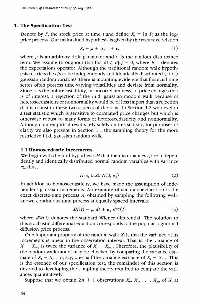
The Review of Financial Studies Spring,1988 1.The Specification Test Denote by P,the stock price at time t and define X,In P,as the log- price process.Our maintained hypothesis is given by the recursive relation X,=4+X,-1+e, (1) where u is an arbitrary drift parameter and e,is the random disturbance term.We assume throughout that for all t,Efe]=0,where E[]denotes the expectations operator.Although the traditional random walk hypoth- esis restricts the e,'s to be independently and identically distributed (i.i.d.) gaussian random variables,there is mounting evidence that financial time series often possess time-varying volatilities and deviate from normality. Since it is the unforecastability,or uncorrelatedness,of price changes that is of interest,a rejection of the i.i.d.gaussian random walk because of heteroscedasticity or nonnormality would be of less import than a rejection that is robust to these two aspects of the data.In Section 1.2 we develop a test statistic which is sensitive to correlated price changes but which is otherwise robust to many forms of heteroscedasticity and nonnormality. Although our empirical results rely solely on this statistic,for purposes of clarity we also present in Section 1.1 the sampling theory for the more restrictive i.i.d.gaussian random walk 1.1 Homoscedastic increments We begin with the null hypothesis H that the disturbances e,are indepen- dently and identically distributed normal random variables with variance a;thus, H:ei.i.d.N(0,2) (2) In addition to homoscedasticity,we have made the assumption of inde pendent gaussian increments.An example of such a specification is the exact discrete-time process X,obtained by sampling the following well- known continuous-time process at equally spaced intervals: dX(t)-udt+o。dw(t) (3) where dw(t)denotes the standard Wiener differential.The solution to this stochastic differential equation corresponds to the popular lognormal diffusion price process. One important property of the random walk X,is that the variance of its increments is linear in the observation interval.That is,the variance of X,-X,-2 is twice the variance of X,-X-1.Therefore,the plausibility of the random walk model may be checked by comparing the variance esti- mate of X,-X,-1 to,say,one-half the variance estimate of X,-X,-2.This is the essence of our specification test;the remainder of this section is devoted to developing the sampling theory required to compare the vari- ances quantitatively. Suppose that we obtain 2n +1 observations X,Xi,...,Xam of X,at 44
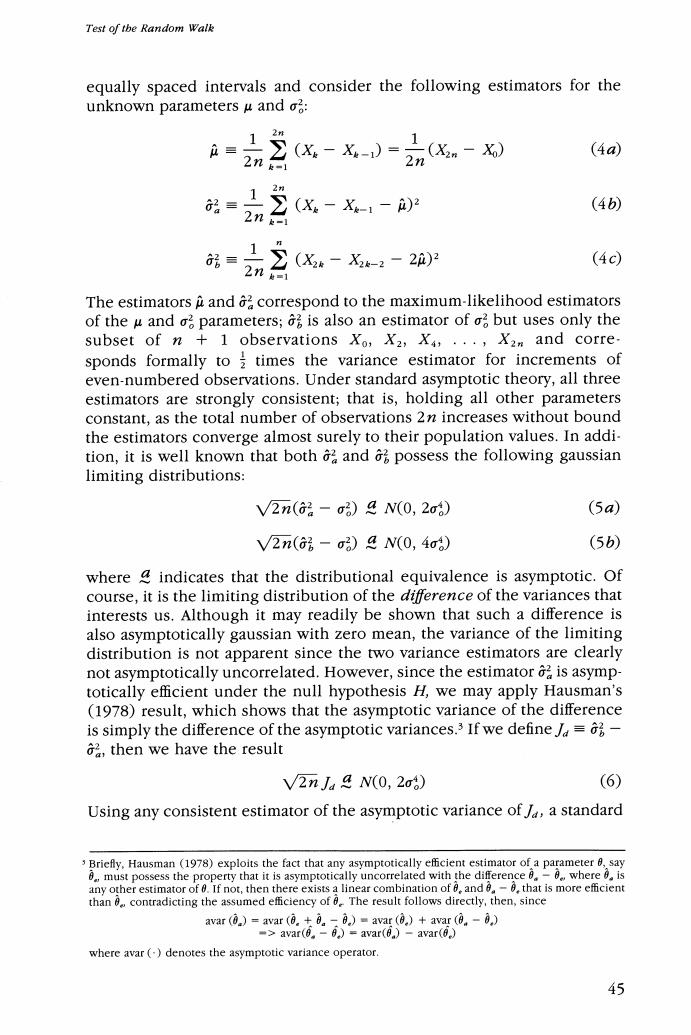
Test of tbe Random Walk equally spaced intervals and consider the following estimators for the unknown parameters u and o: 1 2排 (X。-X-)= 1(X2 -X) (4a) 2ne-1 2 品= 2 (4b) 2nk-1 (X。-X-1-)2 2(&-,-2 (4c) 2n0=1 The estimators a and correspond to the maximum-likelihood estimators of the u and o parameters;is also an estimator of o but uses only the subset of n 1 observations Xo,X2,X,...,X2m and corre. sponds formally to times the variance estimator for increments of even-numbered observations.Under standard asymptotic theory,all three estimators are strongly consistent;that is,holding all other parameters constant,as the total number of observations 2n increases without bound the estimators converge almost surely to their population values.In addi- tion,it is well known that both and possess the following gaussian limiting distributions: V2n(2-σ)4N(0,2o) (5a) V2n(3-o)&N(0,4o) (5b) where indicates that the distributional equivalence is asymptotic.Of course,it is the limiting distribution of the difference of the variances that interests us.Although it may readily be shown that such a difference is also asymptotically gaussian with zero mean,the variance of the limiting distribution is not apparent since the two variance estimators are clearly not asymptotically uncorrelated.However,since the estimator is asymp- totically efficient under the null hypothesis H,we may apply Hausman's (1978)result,which shows that the asymptotic variance of the difference is simply the difference of the asymptotic variances.3 If we define=- then we have the result V2n Ja 4 N(0,200) (6) Using any consistent estimator of the asymptotic variance of /a standard Briefy,Hausman (1978)exploits the fact that any asymptotically efficient estimator of a parameter 0,say 8.,must possess the property that it is asymptotically uncorrelated with the difference .-0.where 8.is any other estimator of 0.If not,then there exists a linear combination of and .-8,that is more efficient than 8,contradicting the assumed efficiency of 6.The result follows directly,then,since avar (0)avar (0.0.)=avar (0.)+avar (0-0) -avar(6.-6)=avar()-avar(6.) where avar (denotes the asymptotic variance operator. 45
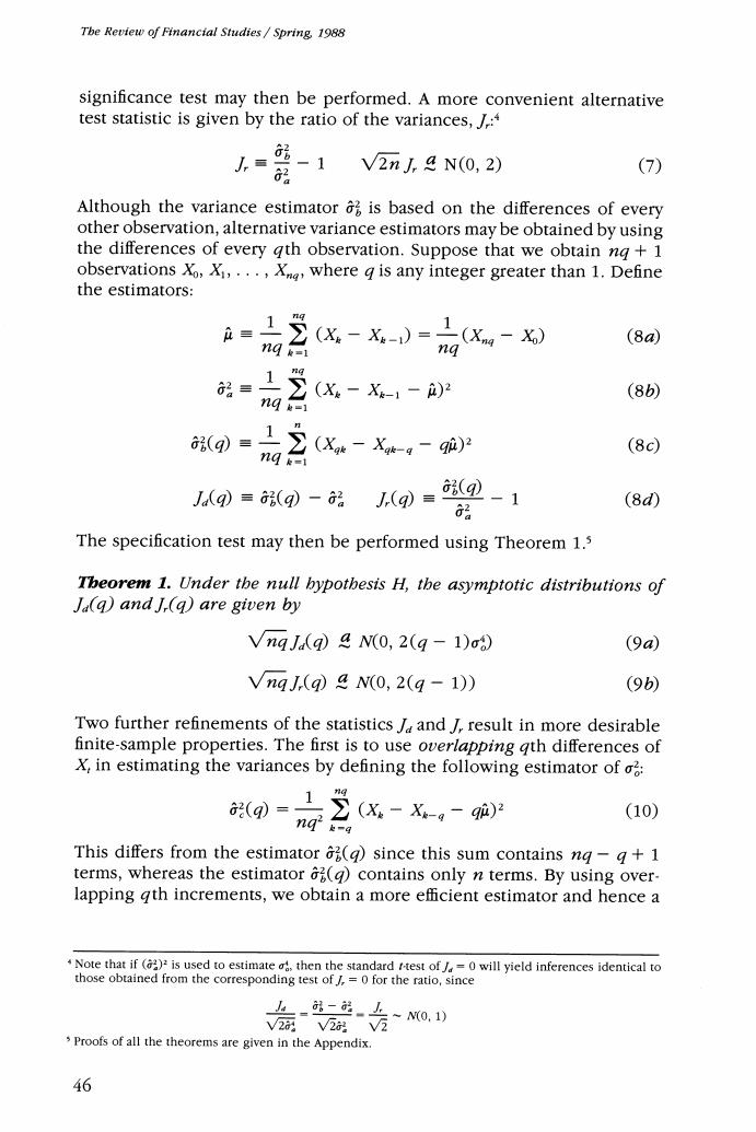
Tbe Review of Financial Studies/Spring,1988 significance test may then be performed.A more convenient alternative test statistic is given by the ratio of the variances,/: 人=-1 2 V2n,4N(0,2) (7) Although the variance estimator is based on the differences of every other observation,alternative variance estimators may be obtained by using the differences of every gth observation.Suppose that we obtain ng +1 observations X,Xi,...,X,where g is any integer greater than 1.Define the estimators: = x-X-)=(x-x (8a 1n☑e= ng 2(x-X&1- (8b) ng (g=22 (Xe-Xk-g-9驴)2 (8c) ng J(q)≡(q)-品 J(g)= 6(①-1 (8d) G经 The specification test may then be performed using Theorem 1.5 Tbeorem 1.Under the null bypotbesis H,the asymptotic distributions of la(q)andI(q)are given by VnqJaq)4 N(0,2(q-1)00) (9a VngJ(q)a N(0,2(g-1)) (9b Two further refinements of the statistics J and /result in more desirable finite-sample properties.The first is to use overlapping qth differences of X,in estimating the variances by defining the following estimator of 2(X-X-,-9m2 (10) This differs from the estimator (g)since this sum contains nq-g+1 terms,whereas the estimator (g)contains only n terms.By using over- lapping gth increments,we obtain a more efficient estimator and hence a Note that if ()is used to estimate,then the standard t-test of=0 will yield inferences identical to those obtained from the corresponding test of/,=0 for the ratio,since 上-i--5~N0,1) V2V2V2 Proofs of all the theorems are given in the Appendix. 46
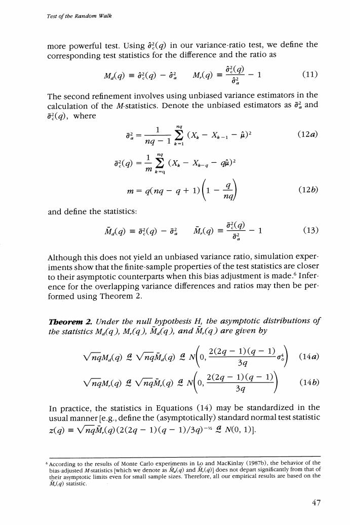
Test of the Random Walk more powerful test.Using 2()in our variance-ratio test,we define the corresponding test statistics for the difference and the ratio as M(q)=2(q)-2M,(q)= (①-1 (11) 62 The second refinement involves using unbiased variance estimators in the calculation of the M-statistics.Denote the unbiased estimators as and (g),where ng-1 觉(X-X-,- (12a) g=1(x-X-,- m m=q(ng- - (12b) and define the statistics: MAq)=(q)- a.()= (①-1 (13) G品 Although this does not yield an unbiased variance ratio,simulation exper- iments show that the finite-sample properties of the test statistics are closer to their asymptotic counterparts when this bias adjustment is made.s Infer- ence for the overlapping variance differences and ratios may then be per- formed using Theorem 2. Tbeorem 2.Under the null bypotbesis H,the asymptotic distributions of the statistics Ma(q),M,(q),Ma(q),and M.(q)are given by VngMa(q)a VngMd(g)4 N0, (29-1)(9-1) (14a 3q VnaM.o Vngn(No,22-D(g-1 (14b) 3q In practice,the statistics in Equations (14)may be standardized in the usual manner [e.g.,define the (asymptotically)standard normal test statistic z(q)=VngM,(q(2(2q-1)(q-1)/3q-N(0,1]: .According to the results of Monte Carlo experiments in Lo and Mackinlay (1987b),the behavior of the bias-adjusted M-statistics [which we denote as M()and M,()]does not depart significantly from that of their asymptotic limits even for small sample sizes.Therefore,all our empirical results are based on the M(g)statistic. 47

The Review of Financial Studies/Spring,1988 To develop some intuition for these variance ratios,observe that for an aggregation value g of 2,the M,()statistic may be reexpressed as 1 M2)=1)-4iaX-X-2+(x.-X-1-2月≥(10(15) Hence,for g=2 the M(g)statistic is approximately the first-order auto- correlation coefficient estimator p(1)of the differences.More generally,it may be shown that M(g)-29-卫1)+2g-262)+…+2(g-1) 2 (16) q q where (k)denotes the kth-order autocorrelation coefficient estimator of the first differences of X.7 Equation (16)provides a simple interpretation for the variance ratios computed with an aggregation value g:They are (approximately)linear combinations of the first g-1 autocorrelation coefficient estimators of the first differences with arithmetically declining weights.8 1.2 Heteroscedastic increments Since there is already a growing consensus among financial economists that volatilities do change over time,?a rejection of the random walk hypothesis because of heteroscedasticity would not be of much interest. We therefore wish to derive a version of our specification test of the random walk model that is robust to changing variances.As long as the increments are uncorrelated,even in the presence of heteroscedasticity the variance ratio must still approach unity as the number of observations increase without bound,for the variance of the sum of uncorrelated increments must still equal the sum of the variances.However,the asymptotic variance of the variance ratios will clearly depend on the type and degree of het- eroscedasticity present.One possible approach is to assume some specific form of heteroscedasticity and then to calculate the asymptotic variance of M,(g)under this null hypothesis.However,to allow for more general forms of heteroscedasticity,we employ an approach developed by White (1980)and by White and Domowitz (1984).This approach also allows us to relax the requirement of gaussian increments,an especially important See Equation (A2-2)in the Appendix. Note the similarity between these variance ratios and the Box-Pierce O-statistic,which is a linear combi- nation of squared autocorrelations with all the weights set identically equal to unity.Although we may expect the finite-sample behavior of the variance ratios to be comparable to that of the o-statistic under the null hypothesis,they can have very different power properties under various alternatives.See Lo and MacKinlay (1987b)for further details. See,for example,Merton (1980),Poterba and Summers (1986),and French,Schwert,and Stambaugh (1987). 48

Test of the Random Walke extension in view of stock returns'well-documented empirical departures from normality.10 Specifically,we consider the null hypothesis H* 1.For all t,E(e)=0,and E(e)=0 for any0. 2.e,}is o-mixing with coefficients (m)of size r/(2r-1)or is a-mixing with coefficients a(m)of size r/(r-1),where r>1,such that for all t and for anyT20,there exists some 6>0 for which E|ee,-,|2+<△<∞ (17) 3.1m2⑨-吃<∞ ng-oo nq t1 4.For all 1,E()=0 for any nonzero jand k wherejk. This null hypothesis assumes that X,possesses uncorrelated increments but allows for quite general forms of heteroscedasticity,including deter ministic changes in the variance (due,for example,to seasonal factors) and Engle's (1982)ARCH processes (in which the conditional variance depends on past information). Since M(g)still approaches zero under H*,we need only compute its asymptotic variance [call it 0()]to perform the standard inferences.We do this in two steps.First,recall that the following equality obtains asymp- totically: M,(q)g】 2(g-卫() (18) =1 q Second,note that under H*(condition 4)the autocorrelation coefficient estimators p(are asymptotically uncorrelated.12 If we can obtain asymp- totic variances (for each of the p()under H*,we may readily calculate the asymptotic variance 0(g)of M(g)as the weighted sum of the 6(p), 10 Of course,second moments are still assumed to be finite;otherwise,the variance ratio is no longer well defined.This rules out distributions with infinite varlance,such as those in the stable Pareto Levy family (with characteristic exponents that are less than 2)proposed by Mandelbrot (1963)and Fama (1965).We do,however,allow for many other forms of leptokurtosis,such as that generated by Engle's (1982) autoregressive conditionally heteroscedastic (ARCH)process. nCondition I is the essential property of the random walk that we wish to test.Conditions 2 and 3 are restrictions on the maximum degree of dependence and heterogeneity allowable while still permitting some form of the law of large numbers and the central limit theorem to obtain.See White (1984)for the precise definitions of and a-mixing random sequences.Condition 4 implies that the sample autocor. relations of e,are asymptotically uncorrelated;this condition may be weakened considerably at the expense of computational simplicity (see note 12). Although this restriction on the fourth cross-moments of e,may seem somewhat unintuitive,it is satisfied for any process with independent increments(regardless of heterogeneity)and also for linear gaussian ARCH processes.This assumption may be relaxed entirely,requiring the estimation of the asymptotic covariances of the autocorrelation estimators in order to estimate the limiting variance 0 of M(g)via relation (18).Although the resulting estimator of would be more complicated than Equation (20),it is conceptually straightforward and may readily be formed along the lines of Newey and West(1987).An even more general (and possibly more exact)sampling theory for the variance ratios may be obtained using the results of Dufour (1981)and Dufour and Roy (1985).Again,this would sacrifice much of the simplicity of our asymptotic results. 49