
An Empirical Evaluation of Accounting Income Numbers STOR Ray Ball;Philip Brown Journal of Accounting Research,Volume 6,Issue 2 (Autumn,1968),159-178. Stable URL: http://links.istor.org/sici?sici=0021-8456%28196823%296%3A2%3C159%3AAEEOA13E2.0.CO%3B2-W Your use of the JSTOR archive indicates your acceptance of JSTOR's Terms and Conditions of Use,available at http://www.jstor.org/about/terms.html.JSTOR's Terms and Conditions of Use provides,in part,that unless you have obtained prior permission,you may not download an entire issue of a journal or multiple copies of articles,and you may use content in the JSTOR archive only for your personal,non-commercial use. Each copy of any part of a JSTOR transmission must contain the same copyright notice that appears on the screen or printed page of such transmission. Journal ofAccounting Research is published by The Institute of Professional Accounting,Graduate School of Business,University of Chicago.Please contact the publisher for further permissions regarding the use of this work.Publisher contact information may be obtained at http://www.jstor.org/journals/grad-uchicago.html. Journal of Accounting Research 1968 The Institute of Professional Accounting,Graduate School of Business,University of Chicago JSTOR and the JSTOR logo are trademarks of JSTOR,and are Registered in the U.S.Patent and Trademark Office. For more information on JSTOR contact jstor-info@umich.edu. ©2003 JSTOR http://www.jstor.org/ Tue Feb1806:46:202003
An Empirical Evaluation of Accounting Income Numbers RAY BALL*and PHILIP BROW N Accounting theorists have generally evaluated the usefulness of account- ing practices by the extent of their agreement with a particular analytic model.The model may consist of only a few assertions or it may be a rigorously developed argument.In each case,the method of evaluation has been to compare existing practices with the more preferable practices im- plied by the model or with some standard which the model implies all practices should possess.The shortcoming of this method is that it ignores a significant source of knowledge of the world,namely,the extent to which the predictions of the model conform to observed behavior. It is not enough to defend an analytical inquiry on the basis that its assumptions are empirically supportable,for how is one to know that a theory embraces all of the relevant supportable assumptions?And how does one explain the predictive powers of propositions which are based on un- verifiable assumptions such as the maximization of utility functions? Further,how is one to resolve differences between propositions which arise from considering different aspects of the world? The limitations of a completely analytical approach to usefulness are il- lustrated by the argument that income numbers cannot be defined sub- stantively,that they lack "meaning"and are therefore of doubtful utility.1 The argument stems in part from the patchwork development of account- *University of Chicago.University of Western Australia.The authors are indebted to the participants in the Workshop in Accounting Research at the Univer- sity of Chicago,Professor Myron Scholes,and Messrs.Owen Hewett and Ian Watts. 1 Versions of this particular argument appear in Canning (1929);Gilman(1939); Paton and Littleton (1940);Vatter (1947),Ch.2;Edwards and Bell (1961),Ch.1; Chambers (1964),pp.267-68;Chambers (1966),pp.4 and 102;Lim (1966),esp.pp.645 and 649;Chambers (1967),pp.745-55;Ijiri (1967),Ch.6,esp.pp.120-31;and Sterling (1967),p.65. 159
160 JOURNAL OF ACCOUNTING RESEARCH,AUTUMN,1968 ing practices to meet new situations as they arise.Accountants have had to deal with consolidations,leases,mergers,research and development,price- level changes,and taxation charges,to name just a few problem areas. Because accounting lacks an all-embracing theoretical framework,dissimi- larities in practices have evolved.As a consequence,net income is an ag- gregate of components which are not homogeneous.It is thus alleged to be a "meaningless"figure,not unlike the difference between twenty-seven tables and eight chairs.Under this view,net income can be defined only as the result of the application of a set of procedures Xi,X2,...}to a set of events Y1,Y2,...}with no other definitive substantive meaning at all. Canning observes: What is set out as a measure of net income can never be supposed to be a fact in any sense at all except that it is the figure that results when the accountant has finished applying the procedures which he adopts.3 The value of analytical attempts to develop measurements capable of definitive interpretation is not at issue.What is at issue is the fact that an analytical model does not itself assess the significance of departures from its implied measurements.Hence it is dangerous to conclude,in the absence of further empirical testing,that a lack of substantive meaning implies a lack of utility. An empirical evaluation of accounting income numbers requires agree- ment as to what real-world outcome constitutes an appropriate test of use- fulness.Because net income is a number of particular interest to investors, the outcome we use as a predictive criterion is the investment decision as it is reflected in security prices.3 Both the content and the timing of existing annual net income numbers will be evaluated since usefulness could be im- paired by deficiencies in either. An Empirical Test Recent developments in capital theory provide justification for selecting the behavior of security prices as an operational test of usefulness.An im- pressive body of theory supports the proposition that capital markets are both efficient and unbiased in that if information is useful in forming capital asset prices,then the market will adjust asset prices to that information quickly and without leaving any opportunity for further abnormal gain. If,as the evidence indicates,security prices do in fact adjust rapidly to new information as it becomes available,then changes in security prices will re- Canning (1920),p.98. 3 Another approach pursued by Beaver (1968)is to use the investment decision, as it is refected in transactions volume,for a predictive criterion. For example,Samuelson (1965)demonstrated that a market without bias in its evaluation of information will give rise to randomly fluctuating time series of prices. See also Cootner (ed.)(1964);Fama (1965);Fama and Blume (1966);Fama,et al. (1967);and Jensen(1968)
EMPIRICAL EVALUATION OF ACCOUNTING INCOME NUMBERS 161 flect the flow of information to the market.5 An observed revision of stock prices associated with the release of the income report would thus provide evidence that the information reflected in income numbers is useful. Our method of relating accounting income to stock prices builds on this theory and evidence by focusing on the information which is unique to a particular firm.6 Specifically,we construct two alternative models of what the market expects income to be and then investigate the market's reac- tions when its expectations prove false. EXPECTED AND UNEXPECTED INCOME CHANGES Historically,the incomes of firms have tended to move together.One study found that about half of the variability in the level of an average firm's earnings per share (EPS)could be associated with economy-wide effects.7 In light of this evidence,at least part of the change in a firm's in- come from one year to the next is to be expected.If,in prior years,the in- come of a firm has been related to the incomes of other firms in a particular way,then knowledge of that past relation,together with a knowledge of the incomes of those other firms for the present year,yields a conditional ex- pectation for the present income of the firm.Thus,apart from confirmation effects,the amount of new information conveyed by the present income number can be approximated by the difference between the actual change in income and its conditional expectation. But not all of this difference is necessarily new information.Some changes in income result from financing and other policy decisions made by the firm. We assume that,to a first approximation,such changes are reflected in the average change in income through time. Since the impacts of these two components of change-economy-wide and policy effects-are felt simultaneously,the relationship must be esti- mated jointly.The statistical specification we adopt is first to estimate,by Ordinary Least Squares (OLS),the coefficients (ai,z)from the linear regression of the change in firm i's income(AIj.+)on the change in the average income of all firms (other than firm j)in the market (AMj.)8 using data up to the end of the previous year (r 1,2,...,-1): △Ii,tr=dit+dAMi,tr十ai,tr T=1,2,…,t-1, (1) s One well documented characteristic of the security market is that useful sources of information are acted upon and useless sources are ignored.This is hardly surpris- ing since the market consists of a large number of competing actors who can gain from acting upon better interpretations of the future than those of their rivals.See,for example,Scholes(1967);and footnote 4 above.This evaluation of the security market differs sharply from that of Chambers (1966,pp.272-73). e More precisely,we focus on information not common to all firms,since some in- dustry effects are not considered in this paper. 7Alternatively,35 to 40 per cent could be associated with effects common to all firms when income was defined as tax-adjusted Return on Capital Employed.[Source: Ball and Brown (1967),Table 4.] 8 We call M a "market index"of income because it is constructed only from firms traded on the New York Stock Exchange
162 RAY BALL AND PHILIP BROWN where the hats denote estimates.The expected income change for firm j in year t is then given by the regression prediction using the change in the average income for the market in year t: △Iit=djt+d2t△Mit. The unexpected income change,or forecast error ()is the actual income change minus expected: a6=△Ir-△1. (2) It is this forecast error which we assume to be the new information con- veyed by the present income number. THE MARKET'S REACTION It has also been demonstrated that stock prices,and therefore rates of return from holding stocks,tend to move together.In one study,it was estimated that about 30 to 40 per cent of the variability in a stock's monthly rate of return over the period March,1944 through December,1960 could be associated with market-wide effects.Market-wide variations in stock returns are triggered by the release of information which concerns all firms. Since we are evaluating the income report as it relates to the individual firm,its contents and timing should be assessed relative to changes in the rate of return on the firm's stocks net of market-wide effects. The impact of market-wide information on the monthly rate of return from investing one dollar in the stock of firm j may be estimated by its predicted value from the linear regression of the monthly price relatives of firm i's common stock1o on a market index of returns:1 9King(1966). 10 The monthly price relative of security j for month m is defined as dividends (dim)+closing price (pi),divided by opening price (pjm): PRm=(pi,m+1十dm)/pm, A monthly price relative is thus equal to the discrete monthly rate of return plus unity;its natural logarithm is the monthly rate of return compounded continuously. In this paper,we assume discrete compounding since the results are easier to inter- pret in that form. 11 Fama,et al.(1967)conclude that "regressions of security on market returns over time are a satisfactory method for abstracting from the effects of general market conditions on the monthly rates of return on individual securities."In arriving at their conclusion,they found that "scatter diagrams for the [returns on]individual securities [vis-a-vis the market return]support very well the regression assumptions of linearity,homoscedasticity,and serial independence."Fama,et al.studied the natural logarithmic transforms of the price relatives,as did King(1966).However, Blume (1968)worked with equation(3).We also performed tests on the alternative specification: ln。(PRm)=bi十b2n。(亿m)+im, (3a) where In.denotes the natural logarithmic function.The results correspond closely with those reported below
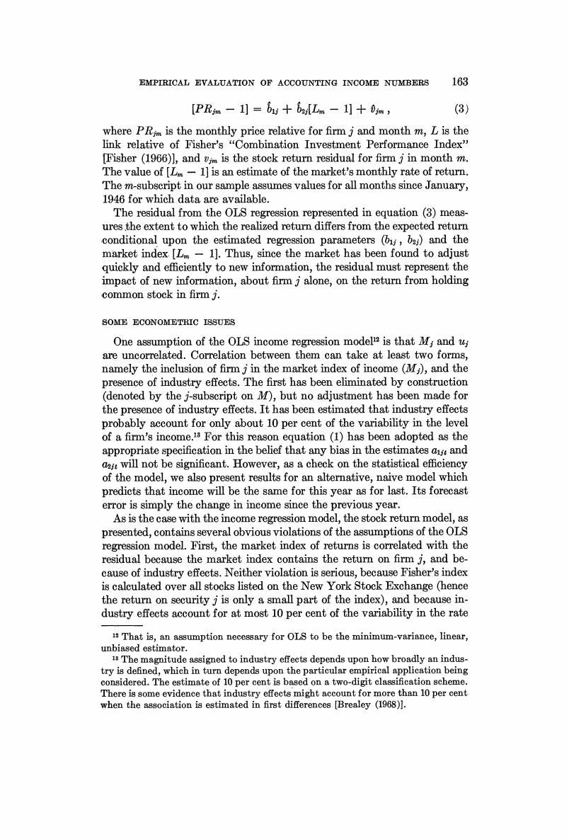
EMPIRICAL EVALUATION OF ACCOUNTING INCOME NUMBERS 163 [PRm-1]=i;+b2d[Lm-1]+0m, (3) where PRim is the monthly price relative for firm j and month m,L is the link relative of Fisher's "Combination Investment Performance Index" [Fisher (1966)],and jm is the stock return residual for firm j in month m. The value of [Lm-1]is an estimate of the market's monthly rate of return. The m-subscript in our sample assumes values for all months since January, 1946 for which data are available. The residual from the OLS regression represented in equation (3)meas- ures the extent to which the realized return differs from the expected return conditional upon the estimated regression parameters (,ba and the market index.[Lm-1].Thus,since the market has been found to adjust quickly and efficiently to new information,the residual must represent the impact of new information,about firm j alone,on the return from holding common stock in firm j. SOME ECONOMETRIC ISSUES One assumption of the OLS income regression model12 is that M;and u; are uncorrelated.Correlation between them can take at least two forms, namely the inclusion of firm j in the market index of income (M;),and the presence of industry effects.The first has been eliminated by construction (denoted by the j-subscript on M),but no adjustment has been made for the presence of industry effects.It has been estimated that industry effects probably account for only about 10 per cent of the variability in the level of a firm's income.1 For this reason equation (1)has been adopted as the appropriate specification in the belief that any bias in the estimates au and aas will not be significant.However,as a check on the statistical efficiency of the model,we also present results for an alternative,naive model which predicts that income will be the same for this year as for last.Its forecast error is simply the change in income since the previous year. As is the case with the income regression model,the stock return model,as presented,contains several obvious violations of the assumptions of the OLS regression model.First,the market index of returns is correlated with the residual because the market index contains the return on firm j,and be- cause of industry effects.Neither violation is serious,because Fisher's index is calculated over all stocks listed on the New York Stock Exchange (hence the return on security j is only a small part of the index),and because in- dustry effects account for at most 10 per cent of the variability in the rate 1That is,an assumption necessary for OLS to be the minimum-variance,linear, unbiased estimator. 1s The magnitude assigned to industry effects depends upon how broadly an indus- try is defined,which in turn depends upon the particular empirical application being considered.The estimate of 10 per cent is based on a two-digit classification scheme. There is some evidence that industry effects might account for more than 10 per cent when the association is estimated in first differences [Brealey (1968)1
164 RAY BALL AND PHILIP BROWN of return on the average stock.14 A second violation results from our predic- tion that,for certain months around the report dates,the expected values of the v,'s are nonzero.Again,any bias should have little effect on the re- sults,inasmuch as there is a low,observed autocorrelation in the ,'s,15 and in no case was the stock return regression fitted over less than 100 observa- tions.16 SUMMARY We assume that in the unlikely absence of useful information about a particular firm over a period,its rate of return over that period would re- flect only the presence of market-wide information which pertains to all firms.By abstracting from market effects [equation (3)]we identify the effect of information pertaining to individual firms.Then,to determine if part of this effect can be associated with information contained in the firm's accounting income number,we segregate the expected and unexpected elements of income change.If the income forecast error is negative (that is, if the actual change in income is less than its conditional expectation),we define it as bad news and predict that if there is some association between accounting income numbers and stock prices,then release of the income number would result in the return on that firm's securities being less than 14 The estimate of 10 per cent is due to King (1966).Blume(1968)has recently questioned the magnitude of industry effects,suggesting that they could be somewhat less than 10 per cent.His contention is based on the observation that the significance attached to industry effects depends on the assumptions made about the parameters of the distributions underlying stock rates of return. 18 See Table 4,below. Fama,et al.(1967)faced a similar situation.The expected values of the stock return residuals were nonzero for some of the months in their study.Stock return regressions were calculated separately for both exclusion and inclusion of the months for which the stock return residuals were thought to be nonzero.They report that both sets of results support the same conclusions. An alternative to constraining the mean v;to be zero is to employ the Sharpe Capi- tal Asset Pricing Model [Sharpe (1964)]to estimate (3b): PRim -RFm-1 =bii+bsj [Lm RFm -1]vim, (3b) where RF is the risk-free ex ante rate of return for holding period m.Results from estimating (3b)(using U.S.Government Bills to measure RF and defining the abnor- mal return for firm j in month m now as biim)are essentially the same as the results from (3). Equation(3b)is still not entirely satisfactory,however,since the mean impact of new information is estimated over the whole history of the stock,which covers at least 100 months.If(3b)were fitted using monthly data,a vector of dummy variables could be introduced to identify the fiscal year covered by the annual report,thus permitting the mean residual to vary between fiscal years.The impact of unusual information received in month m of year t would then be estimated by the sum of the constant,the dummy for year t,and the calculated residual for month m and year t. Unfortunately,the efficiency of estimating the stock return equation in this partic- ular form has not been investigated satisfactorily,hence our report will be confined to the results from estimating (3)
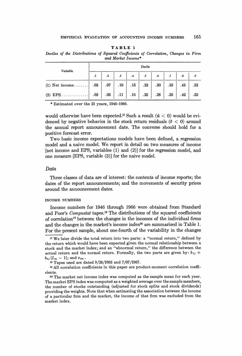
EMPIRICAL EVALUATION OF ACCOUNTING INCOME NUMBERS 165 TABLE 1 Deciles of the Distributions of Squared Coefficients of Correlation,Changes in Firm and Market Income* Decile Variable 3 6 2 9 (1)Net income........ .03 .07 .10 .15 .23 .30 .35 .43 .52 (2)EPS... .02 .05 ,11 .16 .23 .28 .35 .42 .52 Estimated over the 21 years,1946-1966 would otherwise have been expected.17 Such a result (<0)would be evi- denced by negative behavior in the stock return residuals(<0)around the annual report announcement date.The converse should hold for a positive forecast error. Two basic income expectations models have been defined,a regression model and a naive model.We report in detail on two measures of income [net income and EPS,variables (1)and (2)]for the regression model,and one measure [EPS,variable(3)]for the naive model. Data Three classes of data are of interest:the contents of income reports;the dates of the report announcements;and the movements of security prices around the announcement dates. INCOME NUMBERS Income numbers for 1946 through 1966 were obtained from Standard and Poor's Compustat tapes.18 The distributions of the squared coefficients of correlation'between the changes in the incomes of the individual firms and the changes in the market's income index20 are summarized in Table 1. For the present sample,about one-fourth of the variability in the changes We later divide the total return into two parts:a "normal return,"defined by the return which would have been expected given the normal relationship between a stock and the market index;and an "abnormal return,"the difference between the actual return and the normal return.Formally,the two parts are given by:b1;+ bi[Lm-1];and im· 18 Tapes used are dated 9/28/1965 and 7/07/1967. 19 All correlation coefficients in this paper are product-moment correlation coeffi- cients. 20 The market net income index was computed as the sample mean for each year. The market EPS index was computed as a weighted average over the sample members, the number of stocks outstanding (adjusted for stock splits and stock dividends) providing the weights.Note that when estimating the association between the income of a particular firm and the market,the income of that firm was excluded from the market index
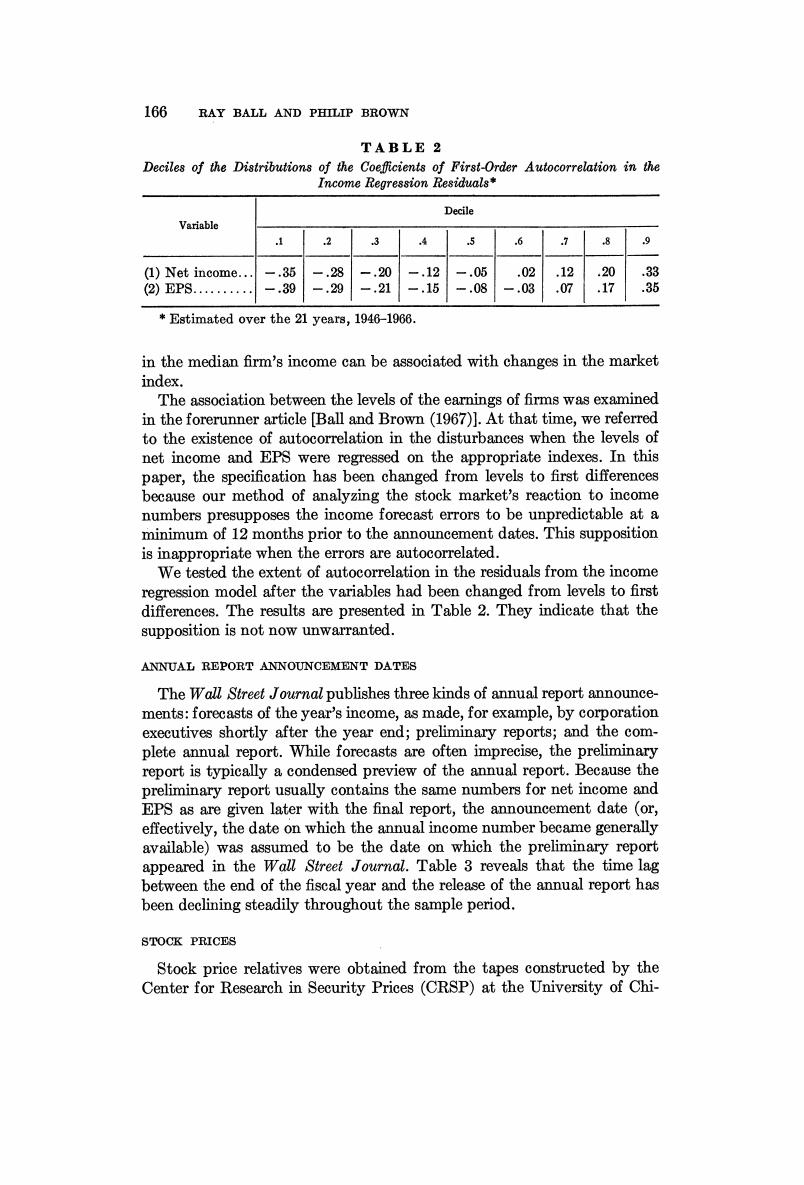
166 RAY BALL AND PHILIP BROWN TABLE 2 Deciles of the Distributions of the Coefficients of First-Order Autocorrelation in the Income Regression Residuals* Decile Variable 1 2 3 .4 .5 .6 8 9 (1)Net income. -.35 =.28 -.20 -.12 -.05 .02 .12 .20 .33 (2)EP8.. .39 -.29 -.21 -.15 -.08 -.03 .07 .17 .35 Estimated over the 21 years,1946-1966. in the median firm's income can be associated with changes in the market index. The association between the levels of the earnings of firms was examined in the forerunner article [Ball and Brown(1967)].At that time,we referred to the existence of autocorrelation in the disturbances when the levels of net income and EPS were regressed on the appropriate indexes.In this paper,the specification has been changed from levels to first differences because our method of analyzing the stock market's reaction to income numbers presupposes the income forecast errors to be unpredictable at a minimum of 12 months prior to the announcement dates.This supposition is inappropriate when the errors are autocorrelated. We tested the extent of autocorrelation in the residuals from the income regression model after the variables had been changed from levels to first differences.The results are presented in Table 2.They indicate that the supposition is not now unwarranted. ANNUAL REPORT ANNOUNCEMENT DATES The Wall Street Journal publishes three kinds of annual report announce- ments:forecasts of the year's income,as made,for example,by corporation executives shortly after the year end;preliminary reports;and the com- plete annual report.While forecasts are often imprecise,the preliminary report is typically a condensed preview of the annual report.Because the preliminary report usually contains the same numbers for net income and EPS as are given later with the final report,the announcement date (or, effectively,the date on which the annual income number became generally available)was assumed to be the date on which the preliminary report appeared in the Wall Street Journal.Table 3 reveals that the time lag between the end of the fiscal year and the release of the annual report has been declining steadily throughout the sample period. STOCK PRICES Stock price relatives were obtained from the tapes constructed by the Center for Research in Security Prices(CRSP)at the University of Chi-
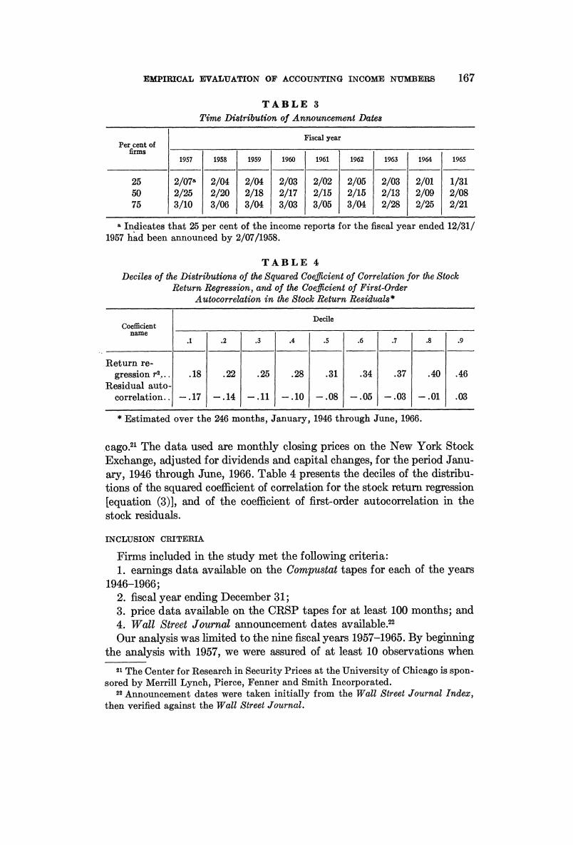
EMPIRICAL EVALUATION OF ACCOUNTING INCOME NUMBERS 167 TABLE 3 Time Distribution of Announcement Dates Fiscal year Per cent of firms 1957 1958 1959 1960 1961 1962 1963 1964 1965 25 2/07 2/04 2/04 2/03 2/02 2/05 2/03 2/01 1/31 2/25 2/20 2/18 2/17 2/15 2/15 2/13 2/09 2/08 的 3/10 3/06 3/04 3/03 3/05 3/04 2/28 2/25 2/21 .Indicates that 25 per cent of the income reports for the fiscal year ended 12/31/ 1957 had been announced by 2/07/1958 TABLE 4 Deciles of the Distributions of the Squared Coefficient of Correlation for the Stock Return Regression,and of the Coeficient of First-Order Autocorrelation in the Stock Return Residuals* Decile name 1 2 3 4 5 .6 7 8 .9 Return re- gression r2.. .18 .22 .25 .28 .31 .34 .37 .40 ,46 Residual auto correlation. -.17 -.14 -,11 -.10 -.08 -.05 -.03 -.01 .03 Estimated over the 246 months,January,1946 through June,1966. cago.2 The data used are monthly closing prices on the New York Stock Exchange,adjusted for dividends and capital changes,for the period Janu- ary,1946 through June,1966.Table 4 presents the deciles of the distribu- tions of the squared coefficient of correlation for the stock return regression lequation (3)],and of the coefficient of first-order autocorrelation in the stock residuals. INCLUSION CRITERIA Firms included in the study met the following criteria: 1.earnings data available on the Compustat tapes for each of the years 1946-1966; 2.fiscal year ending December 31; 3.price data available on the CRSP tapes for at least 100 months;and 4.Wall Street Journal announcement dates available." Our analysis was limited to the nine fiscal years 1957-1965.By beginning the analysis with 1957,we were assured of at least 10 observations when a The Center for Research in Security Prices at the University of Chicago is spon- sored by Merrill Lynch,Pierce,Fenner and Smith Incorporated. Announcement dates were taken initially from the Wall Street Journal Index, then verified against the Wall Street Journal