
Implementing Statistical Criteria to Select Return Forecasting Models:What Do We Learn? TOR Peter Bossaerts;Pierre Hillion The Review of Financial Studies,Volume 12,Issue 2 (Summer,1999),405-428. Stable URL: hup://links.jstor.org/sici?sici=0893-9454%28199922%2912%3A2%3C405%3AISCTSR%3E2.0.CO%3B2-K Your use of the JSTOR archive indicates your acceptance of JSTOR's Terms and Conditions of Use,available at http://www.jstor.org/about/terms.html.JSTOR's Terms and Conditions of Use provides,in part,that unless you have obtained prior permission,you may not download an entire issue of a journal or multiple copies of articles,and you may use content in the JSTOR archive only for your personal,non-commercial use. Each copy of any part of a STOR transmission must contain the same copyright notice that appears on the screen or printed page of such transmission. The Review of Financial Studies is published by Oxford University Press.Please contact the publisher for further permissions regarding the use of this work.Publisher contact information may be obtained at http://www.jstor.org/journals/oup.html. The Review of Financial Studies 1999 Oxford University Press JSTOR and the JSTOR logo are trademarks of JSTOR,and are Registered in the U.S.Patent and Trademark Office. For more information on JSTOR contact jstor-info@umich.edu. ©2003 JSTOR http://www.jstor.org/ Mon Feb1718:17:092003
Implementing Statistical Criteria to Select Return Forecasting Models: What Do We Learn? Peter Bossaerts California Institute of Technology Pierre Hillion INSEAD Statistical model selection criteria provide an informed choice of the model with best external(i.e.,out-of-sample)validity.Therefore they guard against overfitting ("data snooping").We implement several model selection criteria in order to verify recent evidence of predictability in excess stock returns and to determine which variables are valuable predictors.We confirm the presence of in-sample predictability in an international stock market dataset,but discover that even the best prediction models have no out-of-sample forecasting power.The failure to detect out-of-sample predictability is not due to lack of power. 1.Introduction Almost all validation of financial theory is based on historical datasets. Take,for instance,the theory of efficient markets.Loosely speaking,it asserts that securities returns must not be predictable from past information. Numerous studies have attempted to verify this theory,and ample evidence of predictability has been uncovered.This has led many to question the validity of the theory. Quite reasonably,some have recently questioned the conclusiveness of such findings,pointing to the fact that they are based on repeated reeval- uation of the same dataset,or,if not the same,at least datasets that cover similar time periods.For instance,Lo and MacKinlay (1990)argue that Address corresponcence to Peter Bossaerts.HSS 228-77.California Institute of Technology,Pasadena, CA 91125.or e-mail:pbs@rioja.caltech.edu.P.Bossaerts thanks First Quadrant for financial support through a grant to the Califoria Institute of Technology.First Quadrant also provided the data that were used in this study.The article was revised in part when the first author was at the Center for Economic Research.Tilburg University.P.Hillion thanks the Hong Kong University of Science and Technology for their hospitality while doing part of the research.Comments from Michel Dacorogna,Rob Engle,Joel Hasbrouck.Andy Lo,P.C.B.Phillips,Richard Roll,Mark Taylor,and Ken West.from two anonymous referees.and the editor(Ravi Jagannathan),as well as seminar participants at the Hong Kong University of Science and Technology.University of California San Diego.University of Califomia Santa Barbara the 1994 NBER Spring Conference on Asset Pricing,the 1994 Western Finance Association Meetings. and the 1995 CEPR/LIFE Conference on International Finance are gratefully acknowledged. The Review of Financial Stdies Summer 1999 Vol.12,No.2,pp.405-428 e 1999 The Society for Financial Studies 0893-9454/99/$1.50

The Review of Financial Smdies /v 12 n 2 1999 the "size effect"in tests of the capital asset pricing model (CAPM)may very well be the result of an unconscious,exhaustive search for a portfolio formation criterion with the aim of rejecting the theory. Repeated visits of the same dataset indeed lead to a problem that statis- ticians refer to as model overfitting [Lo and MacKinlay (1990)called it "data snooping"],that is,the tendency to discover spurious relationships when applying tests that are inspired by evidence from prior visits to the same dataset.There are several ways to address model overfitting.The finance literature has emphasized two approaches.First,one can attempt to collect new data,covering different time periods and/or markets [e.g., Solnik (1993)].Second,standard test sizes can be adjusted for overfitting tendencies.These adjustments are either based on theoretical approxima- tions such as Bonferroni bounds [Foster,Smith,and Whaley (1997)],or on bootstrapping stationary time series [Sullivan,Timmermann,and White (1997)1. The two routes that the finance literature has taken to deal with model overfitting,however,do present some limitations.New,independent data are available only to a certain extent.And adjustment of standard test sizes merely help in correctly rejecting the simple null hypothesis of no rela- tionship.It will provide little information,however,when,in addition,the empiricist is asked to discriminate between competing models under the alternative of the existence of some relationship. In contrast,the statistics literature has long promoted model selection criteria to guard against overfitting.Of these,Akaike's criterion [Akaike (1974)]is probably the best known.There are many others,however,in- spired by different criteria about what constitutes an optimal model (one distinguishes Bayesian and information-theoretic criteria),and with varying degrees of robustness to unit-root nonstationarities in the data. The purpose of this article is to implement several selection criteria from the statistics literature (including our own,meant to correct some well- known small-sample biases in one of these criteria),based on popularity and on robustness to unit roots in the independent variables.The aim is to verify whether stock index returns in excess of the riskfree rate are indeed predictable,as many have recently concluded [e.g.,Fama (1991),Keim and Stambaugh (1986),Campbell (1987),Breen,Glosten,and Jagannathan (1990),Brock,Lakonishok,and LeBaron (1992),Sullivan,Timmermann, and White (1997)]. Our insistence on model selection criteria that are robust to unit-root nonstationarities is motivated by the time-series properties of some candi- date predictors,such as price-earnings ratios,dividend yields,lagged index levels,or even short-term interest rates.These variables are either mani- Foster,Smith,and Whaley (1997)also present simulation-based adjustments. 406
Implementing Statistical Criteria to Select Return Forecasting Models festly nonstationary,or,if not,their behavior is close enough to unit-root nonstationary for small-sample statistics to be affected. We study an international sample of excess stock returns and candidate predictors which First Quadrant was kind enough to release to us.The time period nests that of another international study,Solnik(1993).Therefore, we also provide diagnostic tests that compare the two datasets (which are based on different sources). We discover ample evidence of predictability,confirming the conclusion of studies that were not based on formal model selection criteria.Usually only a few standard predictors are retained,however.Some of these are unit- root nonstationary (e.g.,dividend yield).Multiple lagged bond or stock returns are at times included,effectively generating the moving-average predictors that have become popular in professional circles lately [see also Brock,Lakonishok,and LeBaron (1992)and Sullivan,Timmermann,and White(1997)]. Formal model selection criteria guard against overfitting.The ultimate purpose is to obtain the model with the best external validity.In the context of prediction,this means that the retained model should provide good out- of-sample predictability.We test this on our dataset of international stock returns. Overall,we find no out-of-sample predictability.More specifically,none of the models that the selection criteria chose generates significant predic- tive power in the 5-year period beyond the initial ("training)sample.This conclusion is based on an SUR test of the slope coefficients in out-of-sample regressions of outcomes onto predictions across the different stock markets. The failure to detect out-of-sample predictability cannot be attributed to lack of power.Schwarz's Bayesian criterion,for instance,discovers predictabil- ity in 9 of 14 markets,with an average R2 of the retained models of 6%. Out of sample,however,none of the retained models generates significant forecasting power.Even with only nine samples of 60 months each,chances that this would occur if 6%were indeed the true R2 are less than I in 333. The poor external validity of the prediction models that formal model selection criteria chose indicates model nonstationarity:the parameters of the"best"prediction model change over time.It is an open question why this is.One potential explanation is that the "correct"prediction model is actually nonlinear,while our selection criteria chose exclusively among linear models.Still,these criteria pick the best linear prediction model:it is surprising that even this best forecaster does not work out of sample. As an explanation for the findings,however,model nonstationarity lacks economic content.It begs the question as to what generates this nonsta- tionarity.Pesaran and Timmermann(1995)also noticed that prediction per- formance improves if one switches models over time.They suggest that it reflects learning in the marketplace.Bossaerts(1997)investigates this possi- bility theoretically.He proves that evidence of predictability will disappear 407
The Review of Financial Smdies /v12 n 2 1999 entirely out of sample if the market learns on the basis of Bayesian updating rules.In other words,Bayesian learning could explain our findings. The remainder of this article is organized as follows.The next section introduces model selection criteria.Section 3 describes the dataset.Section 4 presents the results.Section 5 discusses the power of the out-of-sample prediction tests.Section 6 concludes.There are three appendixes.They discuss technical issues and list the data sources. 2.Model Selection Criteria Formal model selection criteria have long been considered in the statistics literature in order to select the "best"model among a set of candidate models.Statisticians realized that there is a tendency to overfit,and hence that the model that has the highest in-sample explanatory power usually does not have the highest external validity (i.e.,out-of-sample fit).Several criteria were developed,starting from particular decision criteria,Bayesian or information theoretic. We decided to pick several model selection criteria in our study of the predictability of excess stock returns.Each has its merit,and many are robust to the presence of unit roots in the candidate predictors.It is not appropriate to discuss here the advantages and shortcomings of the retained selection criteria.Suffice it to mention that all selection criteria contributed uniformly to the main conclusions of this article. Formally,we use statistical criteria and T observations to select among K linear models that predict the market's excess return,r(t =1,...,T).The models differ in terms of the content and dimension of the prediction vector. Let p*denote the dimension for model k (k =1....,K).The prediction vector of this model for the rth returnr is obtained by dropping all but p elements from the vector of all possible predictors,x,-1.x-I includes an intercept as one of the predictors,as well as variables such as the short-term Treasury bill yield,etc.(We will be explicit later on.)Letting o*denote its coefficient vector,model k can be written as n=0x1+e, (1) with E[ef ]=0,Elef]=0. In the first model,with k =1,we included only the intercept.(Hence, p=1.)This way,selection criteria are allowed to decide in favor of no predictabiliry,beyond a constant.The latter is usually interpreted as a (fixed)risk premium.This option is important.Indeed,the original goal of this study was to verify whether the evidence of return predictability would still emerge if examined with formal selection criteria. Each selection criterion chooses among the K possible model specifi- cations.We will use the notation k*to denote the preferred model.Seven 408

Implementing Statistical Criteria to Select Return Forecasting Models model selection criteria were employed:the adjusted R2,Akaike's infor- mation criterion [AIC;Akaike (1974)],Schwarz's criterion [a Bayesian information criterion,BIC;Schwarz (1978)],the Fisher information crite- rion [FIC;Wei(1992)],the posterior information criterion [PIC;Phillips and Ploberger (1996)],Rissanen's predictive least squares criterion [PLS; Rissanen (1986a)],2 and our adjustment to correct well-known biases of the latter,PLS-MDC. Appendix A provides formal definitions of each of these criteria.The adjusted R2,AIC,and BIC were chosen on the basis of their popularity; FIC,PIC,PLS,and PLS-MDC were chosen because of their robustness in the face of unit-root nonstationarities. PLS-MDC is new and hence needs to be motivated further.It is based on a technique to estimate the dimension of the state vector in Markov models,referred to as Markov dimension criterion (MDC).MDC chooses the dimension of the state vector by investigating the out-of-sample mean square prediction error of rolling regressions that are run on the basis of various subsets of past information. In conjunction with PLS,MDC provides a correction for small-sample biases.PLS chooses models on the basis of the out-of-sample mean square prediction error of one rolling regression that uses all past observations. Rissanen (1986a)suggested this selection criterion,but observed that it is biased in small samples in favor of picking the model with the least possible variables [see also the evidence in Wei (1992)].The underfitting is due to the noise introduced by the error in the predictions of early observations in the sample.These predictions are unreliable because they are based on very few prior observations (remember that model estimates in PLS are computed only from prior observations).The fewer parameters to be esti- mated,however,the lower the prediction noise of those early observations. Because of the lower noise level,PLS tends to prefer models with fewer parameters,that is,with less explanatory variables. In PLS-MDC,we consider the performance of the same models where parameter estimates are not only based on all previous observations,but on different subsamples as well,where we drop observations that reach a certain age.In other words,while PLS is based on expanding-window estimation, PLS-MDC also considers estimates based on windows of fixed size.PLS- MDC effectively penalizes models where excluded variables are still heavily correlated with future prediction errors,indicating that the prediction vector was chosen to be too small.Since a formal discussion of PLS-MDC distracts from the main points of this article,it is delegated to an appendix.The interested reader can consult Appendix B. 2 PLS is based on Rissanen's earlier idea of minimum descriptive length [Rissanen (1986b)]:see also Kavalieris (1989). 409
The Review of Financial Studies /v 12n 2 1999 As mentioned before,the purpose of statistical model selection criteria is to avoid overfitting.The model specification that fits the data best(minimum in-sample forecast error)is not necessarily chosen.In contrast,the retained model will have maximum external validity.In our context of return pre- diction,this means that the preferred model will have best out-of-sample forecasting performance. We decided to verify the external validity of formal model selection whenever k*>1.All models with index(k)larger than one contain at least one nontrivial forecasting variable.When one of them is chosen,the model selection criterion clearly supports predictability.To assess the external validity of such a conclusion,we ran a test on a sample that postdated the sample on which we based the model choice.To avoid confusion we will refer to the original sample on which model choice was based as the training sample.The sample that was used to check for external validity will be called the testing sample.The latter has size n,and its elements are indexed tT+1,...,T+n. External validation is investigated by projecting the market's excess re- turn,r,onto our forecast,-1.-1 is obtained from model k*,as follows: -1=1x二 (2) where is the OLSestimate of,based on the pairs ()observed over r =1....t-1.We estimate the slope coefficient in =Q+Bz1-I+, (3) from the observations indexed tT+1,...,T+n.We use the OLS estimate of B to compute a standard t-ratio,and refer to the standard normal distribution to determine p-levels.External validity is confirmed if p-levels are low,say,below 0.05. Notice that we did not adjust the t-ratio for error in the estimation of the parameters of the prediction model.Asymptotically,such an adjustment is not necessary,because we force the precision of the parameter estimates to increase as we advance through the testing sample.See also West(1996). Unfortunately,small-sample corrections are not available and would be complicated by the unit-root nature of some of the predictors. 3.The Data We investigated the predictability of the 1-month local-currency excess stock return for 14 countries.3 Our forecasts of the market's excess return is based on (a subset of)the following predictors:a January dummy;the Results can be expected to be different if excess stock returns are converted to a common currency.in which case retums from speculation in the foreign exchange market determine the outcome as well.See, for example,Ferson and Harvey (1993). 410
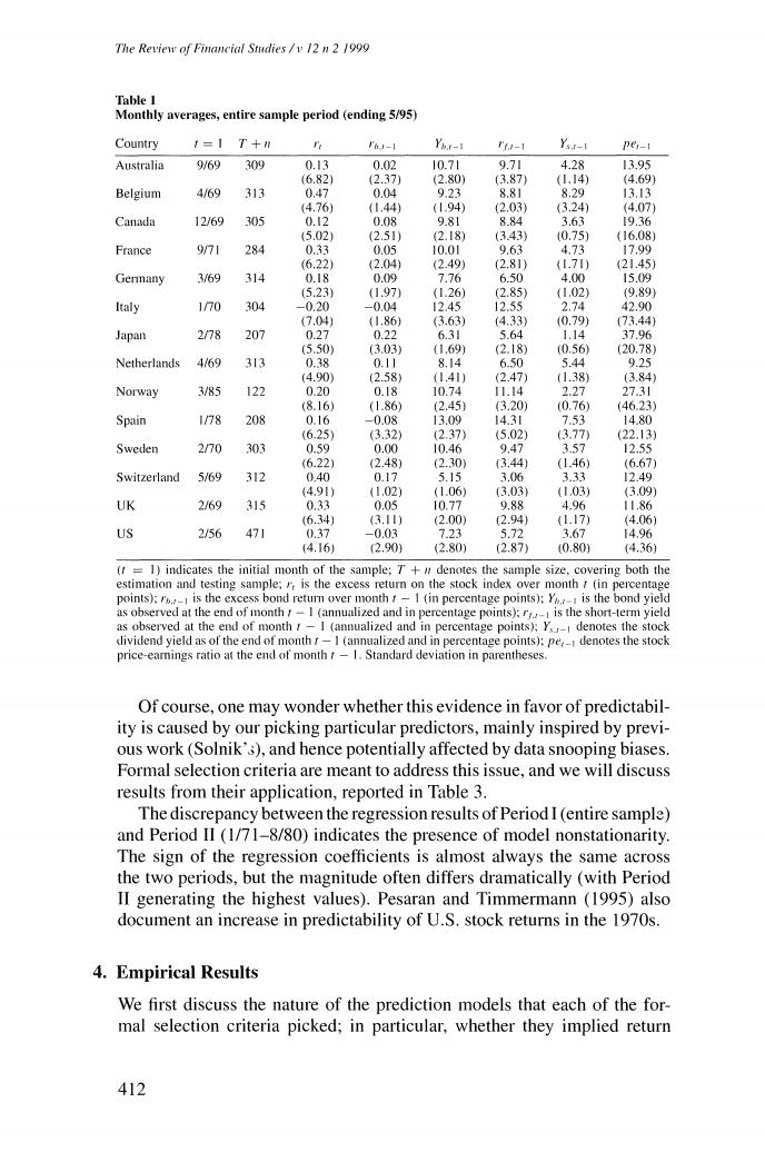
Implementing Statistical Criteria to Select Return Forecasting Models monthly excess stock return,lagged once and twice;a monthly bond excess return,lagged once and twice;*the yield-to-maturity on a representative Treasury bond;the stock market's price level;the yield-to-maturity on a 3- month Treasury bill (also used to compute excess stock and bond returns); the stock market's dividend yield;and the stock market's price-earnings ratio.None of these predictors use information that would not have been available at the moment that future excess stock returns were predicted. Appendix C provides a list of the data sources. Table I displays descriptive statistics of the monthly excess stock returns and the predictors.The lengths of the samples(T+n)run from a minimum of 122 observations (Norway)to a maximum of 471 observations(United States).Returns are expressed in percent per month;yields in percent per year.Table I also lists the beginning of the estimation sample for each country (t =1).Our choice was based on data availability,and hence was purely incidental. To get an idea of the amount of predictability that obtains in this dataset using in-sample statistical analysis,Table 2 lists the results from a regression of monthly excess stock returns (now not expressed in percentage terms) onto (i)an intercept,(ii)a January dummy,(iii)the stock dividend yield, (iv)the short-term interest rate,and (v)the long-term bond yield.Solnik (1993)also reports these estimates,for a similar dataset,but a shorter time period.The results of regressions like the ones reported in Table 2 match those of Solnik when run over his subperiod only (1/71-8/90).There is one exception though:our bond yield has more predictive power than his. A closer look at Table 2 reveals the patterns that Solnik discussed at length:predictability is not uniform across stock markets [R2s are between 2%(Germany)and 9.8%(U.K.)];predictors vary.The well-known nega- tive correlation between excess stock returns and contemporaneous interest rates is significant(at the 1%level)only for Belgium,France,and the United States. An unfortunate choice of subperiod,however,may give one the wrong impression of the amount of predictability.We tried one possible subsample and generated impressive evidence of predictability.Table 2 reports the results from estimation of the same regression over the subperiod 1/71- 8/80(10 years shorter than Solnik's sampling period).They are listed under Period II.The R2s run from a low of 4.4%(Canada)to a high of 36.4% (Belgium)or higher!Overall,the significance of the coefficients in the regression is overwhelming. 4This bond return is actually computed from the yield on a representative Treasury bond and an estimate of the duration.Hence it cannot strictly be considered to be a bond (excess)return.Nevertheless,its computation does not require future information.Therefore it is a proper predictor. 5 Some high R2s may be the result of lack of observations.The highest R2,40%(Spain).is based on a sampling period that runs from 1/78 to 8/80 only.Belgium's high R2.however,is based on a full sample. 411
The Review of Financial Studies /v 12 n 2 1999 Table I Monthly averages,entire sample period (ending 5/95) Country 1=1 T+ I6J-1 Yh.t-1 -1 YsI-I per-1 Australia 9/69 309 0.13 0.02 10.71 9.71 4.28 13.95 (6.82) (2.37 (2.80) (3.87) (1.14) (4.69) Belgium 4/69 313 0.47 0.04 9.23 8.81 8.29 1313 (4.76) (1.44) (1.94) 2.03) (3.24) (4.07) Canada 12/69 305 0.I2 0.08 9.81 8.84 3.63 19.36 (5.02) (2.51) (2.18) (3.43) 0.75) (16.08) France 971 284 0.33 0.05 10.01 9.63 4.73 17.99 (6.22) (2.04) (2.49) (2.81) (1.71) (21.45) Germany 3/69 314 0.18 0.09 7.76 6.50 4.00 15.09 (5.23) (1.97) (1.26) (2.85) (1.02) (9.89) Italy 170 304 -0.20 -0.04 12.45 12.55 2.74 42.90 (7.04 (1.86) (3.63) (4.33) (0.79) (73.44) Japan 2/78 207 0.27 0.22 6.31 5.64 1.14 37.96 (5.50) (3.03 (1.69) (2.18) (0.56 (20.78) Netherlands 4/69 313 0.38 0.11 8.14 6.50 5.44 9.25 14.90 (2.58) (1.41) (2.47) (1.38) (3.84 Norway 3/85 122 0.20 0.18 10.74 11.14 2.27 27.31 (8.16) (1.86) (2.45 (3.20) (0.76) (46.23) Spain 1/78 208 0.16 -0.08 13.09 14.31 7.53 14.80 (6.25 (3.32) (2.37) (5.02) (3.77 (22.13) Sweden 270 303 0.59 0.00 10.46 9.47 3.57 12.55 (6.22) (2.48) (2.30) (3.44) (1.46) (6.67) Switzerland 5/69 312 0.40 0.17 5.15 3.06 3.33 12.49 (4.91) 41.02) (1.06) (3.03) (1.03) (3.09) UK 2/69 315 0.33 0.05 10.77 988 4.96 11.86 (6.34) 3.11) (2.00 (2.94) (1.17) (4.06) US 2/56 471 0.37 -0.03 7.23 5.72 3.67 14.96 (4.16) (2.90) (2.80) (2.87) (0.80) (4.36) (t=1)indicates the initial month of the sample:7+#denotes the sample size,covering both the estimation and testing sample:is the excess return on the stock index over month t(in percentage points):is the excess bond return over month t-I (in percentage points);Y is the bond yield as observed at the end of month /-I (annualized and in percentage points);r,is the short-term yield as observed at the end of month r-I (annualized and in percentage points);Y denotes the stock dividend yield as of the end of month f-I (annualized and in percentage points):pe,_denotes the stock price-earnings ratio at the end of month t-1.Standard deviation in parentheses Of course,one may wonder whether this evidence in favor of predictabil- ity is caused by our picking particular predictors,mainly inspired by previ- ous work (Solnik'3),and hence potentially affected by data snooping biases. Formal selection criteria are meant to address this issue,and we will discuss results from their application,reported in Table 3. The discrepancy between the regression results of Period I(entire sample) and Period II (1/71-8/80)indicates the presence of model nonstationarity. The sign of the regression coefficients is almost always the same across the two periods,but the magnitude often differs dramatically (with Period II generating the highest values).Pesaran and Timmermann (1995)also document an increase in predictability of U.S.stock returns in the 1970s. 4.Empirical Results We first discuss the nature of the prediction models that each of the for- mal selection criteria picked;in particular,whether they implied return 412

Implementing Statistical Criteria to Select Return Forecasting Models Table 2 OLS regressions of monthly excess stock returns on a subset of predictors,various sample periods Country Predicturs Intercept Januiry Diviulenl Shurt-em k dummy yiekl yield Yield 1 1 1 -4 147 10139 - -,177 006533125 22 L.7) 40016 22 C42 f5) NL4K125 (INKO9I CLOU 01I Belgium -01 3锅 f115 4 I线 -41211 -01531 0014 0n1656 364 0145 1012231D111 111 116h I1联I25) 非NI57h cLUIOL jo5) n010DE -(H9 -06 005 05 1m12 0f9 1,23) ( 0012 114界影 KHAKI79) .2 00104 Frarce 0正 -431 2 041 L属 5 -4MI72 -一.N省N 056 -000川a9 137 19) M44)0D15 1213 A131) AN65) NkINI203 ,H3 00m6 00s11 414N2 -40127 057 3 作N1g 4N171 4M21 -4北15 -1m115 候 125 2 3 400129 13 7) 082> y 儿2 -.w7 40 (1AKH42 -KI3 -I.IKHIR -.1m87 L21 0[35 2 41K2 GM251 c030 h 101213 rltINI64) (NM7] (H22) .m251 0004) 1016 Japan 0.3 245 a015 -.H角 DHI3 -.1417 一.IMA角 一Mw6 46 11142125 315 (. .1.321 1414 5 e4场h CD 133II 40078 NAKI54) 5 125 .1 212 (.I (3打4011 l0I+1 GMIKI351 值.MM口3)HI1) D19判 RLXKL7 K场) .131 NO 29 NO .13折 NO 镇3H NO -4165 NO NO 141 B16小 0311i (MI179) Spamn -1X4M12 -B.M -.345 -.2 2 1159 H N 71 1(1X11K> 2 .N21 C11M51151 1 1w559 0015 Swedea -54 位6 31 ,IM29 D293 -位D11 -D54 .WL58 -1川粥 A51 INIX 40D271 i126 113 (DIN2271 位制 DmIXI 40n1 N54N101 NANI5S) 3 2 15到 CIDPIN1 2 111 KIINIW (米 .4N.9) UK D 000 -几I1 LXH1 11KSI D233 DD196 -1022 一 -INMKI -1MN33 界 123 0261 008211tH5) 0251 5明 (I821 4只)4非 001 C.W43 .A州微I与 你 -Dn0x -0017 4KIR 0川 DD115 D0005 -00M -n091 N31 IINIL6 ,7 172 4251 1AM7) . 3 yieldare inmlized and exprexd in percentage terms.Unlike in Tahle 1.thte depencknt viiable.the ntomthly excess stek retumm ix not expressedl in percentagte puints NO na olvervatiuns int peried 1l. predictability.Subsequently,we report tests of the external validity of the selected models(whenever they did imply return predictability in-sample). The estimation sample runs until 5/90.The testing sample covers the re- maining period:6/90-5/95 (hence,n =60). 4.1 Retained Forecasting Models The seven model selection criteria were allowed to pick a suitable prediction model based on the 10 predictors listed in Table 1,as well as a constant(the intercept in the linear prediction model).As mentioned before,predictability is decided against whenever only the constant is retained.The parameters in the prediction models were estimated with OLS. Table 3 displays the composition of the linear prediction model preferred by each of the selection criteria.A zero indicates that the corresponding variable was discarded,a one indicates that the variable was kept.The following facts stand out when looking at this table. The adjusted R2 almost invariably selects a model with more predic- tors than other criteria.This overfitting occurs despite the (admittedly ad hoc)adjustment for the loss of degrees of freedom when regressors are added.In the case of the United States,for instance,the adjusted R2 413