Returns to Buying Winners and Selling Losers:Implications for Stock Market Efficiency STOR Narasimhan Jegadeesh;Sheridan Titman The Journal of Finance,Volume 48,Issue 1 (Mar.,1993),65-91. Stable URL: hup://links.jstor.org/sici?sici=0022-1082%28199303%2948%3A1%3C65%3ARTBWAS%3E2.0.CO%3B2-Y Your use of the JSTOR archive indicates your acceptance of JSTOR's Terms and Conditions of Use,available at http://www.istor.org/about/terms.html.JSTOR's Terms and Conditions of Use provides,in part,that unless you have obtained prior permission,you may not download an entire issue of a journal or multiple copies of articles,and you may use content in the JSTOR archive only for your personal,non-commercial use. Each copy of any part of a STOR transmission must contain the same copyright notice that appears on the screen or printed page of such transmission. The Journal of Finance is published by American Finance Association.Please contact the publisher for further permissions regarding the use of this work.Publisher contact information may be obtained at http://www.jstor.org/journals/afina.html. The Journal of Finance 1993 American Finance Association JSTOR and the JSTOR logo are trademarks of JSTOR,and are Registered in the U.S.Patent and Trademark Office. For more information on JSTOR contact jstor-info@umich.edu. ©2003 JSTOR http://www.jstor.org/ Tue Feb1801:56:402003
THE JOURNAL OF FINANCE.VOL.XLVIII,NO.1.MARCH 1993 Returns to Buying Winners and Selling Losers:Implications for Stock Market Efficiency NARASIMHAN JEGADEESH and SHERIDAN TITMAN* ABSTRACT This paper documents that strategies which buy stocks that have performed well in the past and sell stocks that have performed poorly in the past generate significant positive returns over 3-to 12-month holding periods.We find that the profitability of these strategies are not due to their systematic risk or to delayed stock price reactions to common factors.However,part of the abnormal returns generated in the first year after portfolio formation dissipates in the following two years.A similar pattern of returns around the earnings announcements of past winners and losers is also documented. A POPULAR VIEW HELD by many journalists,psychologists,and economists is that individuals tend to overreact to information.A direct extension of this view,suggested by De Bondt and Thaler(1985,1987),is that stock prices also overreact to information,suggesting that contrarian strategies (buying past losers and selling past winners)achieve abnormal returns.De Bondt and Thaler (1985)show that over 3-to 5-year holding periods stocks that per- formed poorly over the previous 3 to 5 years achieve higher returns than stocks that performed well over the same period.However,the interpretation of the De Bondt and Thaler results are still being debated.Some have argued that the De Bondt and Thaler results can be explained by the systematic risk of their contrarian portfolios and the size effect.?In addition,since the long-term losers outperform the long-term winners only in Januaries,it is unclear whether their results can be attributed to overreaction. "Jegadeesh is from the Anderson Graduate School of Management,UCLA.Titman is from Hong Kong University of Science and Technology and the Anderson Graduate School of Manage- ment,UCLA.We would like to thank Kent Daniel,Ravi Jagannathan,Richard Roll,Hans Stoll, Rene Stulz,and two referees.We also thank participants of the Johnson Symposium held at the University of Wisconsin at Madison and seminar participants at Harvard,SMU,UBC,UCLA, Penn State,University of Michigan,University of Minnesota,and York University for helpful comments,and Juan Siu and Kwan Ho Kim for excellent research assistance. See for example,the academic papers by Kahneman and Tversky (1982),De Bondt and Thaler (1985)and Shiller (1981). See for example,Chan (1988),Ball and Kothari(1989),and Zarowin (1990).For an alternate view,see the recent paper by Chopra,Lakonishok,and Ritter(1992). 65
66 The Journal of Finance More recent papers by Jegadeesh (1990)and Lehmann (1990)provide evidence of shorter-term return reversals.These papers show that contrarian strategies that select stocks based on their returns in the previous week or month generate significant abnormal returns.However,since these strate- gies are transaction intensive and are based on short-term price movements, their apparent success may reflect the presence of short-term price pressure or a lack of liquidity in the market rather than overreaction.Jegadeesh and Titman (1991)provide evidence on the relation between short-term return reversals and bid-ask spreads that supports this interpretation.In addition, Lo and MacKinlay (1990)argue that a large part of the abnormal returns documented by Jegadeesh and Lehmann is attributable to a delayed stock price reaction to common factors rather than to overreaction. Although contrarian strategies have received a lot of attention in the recent academic literature,the early literature on market efficiency focused on relative strength strategies that buy past winners and sell past losers.Most notably,Levy(1967)claims that a trading rule that buys stocks with current prices that are substantially higher than their average prices over the past 27 weeks realizes significant abnormal returns.Jensen and Bennington (1970), however,point out that Levy had come up with his trading rule after examining 68 different trading rules in his dissertation and because of this express skepticism about his conclusions.Jensen and Bennington analyze the profitability of Levy's trading rule over a long time period that was,for the most part,outside Levy's original sample period.They find that in their sample period Levy's trading rule does not outperform a buy and hold strategy and hence attribute Levy's result to a selection bias. Although the current academic debate has focused on contrarian rather than relative strength trading rules,a number of practitioners still use relative strength as one of their stock selection criteria.For example,a majority of the mutual funds examined by Grinblatt and Titman(1989,1991) show a tendency to buy stocks that have increased in price over the previous quarter.In addition,the Value Line rankings are known to be based in large part on past relative strength.The success of many of the mutual funds in the Grinblatt and Titman sample and the predictive power of Value Line rankings(see Copeland and Mayers (1982)and Stickel (1985))provide sug- gestive evidence that the relative strength strategies may generate abnormal returns. How can we reconcile the success of Value Line rankings and the mutual funds that use relative strength rules with the current academic literature that suggests that the opposite strategy generates abnormal returns?One possibility is that the abnormal returns realized by these practitioners are either spurious or are unrelated to their tendencies to buy past winners.A second possibility is that the discrepancy is due to the difference between the time horizons used in the trading rules examined in the recent academic papers and those used in practice.For instance,the above cited evidence favoring contrarian strategies focuses on trading strategies based on either
Returns to Buying Winners and Selling Losers 67 very short-term return reversals (1 week or 1 month),or very long-term return reversals(3 to 5 years).However,anecdotal evidence suggests that practitioners who use relative strength rules base their selections on price movements over the past 3 to 12 months.3 This paper provides an analysis of relative strength trading strategies over 3-to 12-month horizons.Our analy- sis of NYSE and AMEX stocks documents significant profits in the 1965 to 1989 sample period for each of the relative strength strategies examined.We provide a decomposition of these profits into different sources and develop tests that allow us to evaluate their relative importance.The results of these tests indicate that the profits are not due to the systematic risk of the trading strategies.In addition,the evidence indicates that the profits cannot be attributed to a lead-lag effect resulting from delayed stock price reactions to information about a common factor similar to that proposed by Lo and MacKinlay (1990).The evidence is,however,consistent with delayed price reactions to firm-specific information. Further tests suggest that part of the predictable price changes that occur during these 3-to 12-month holding periods may not be permanent.The stocks included in the relative strength portfolios experience negative abnor- mal returns starting around 12 months after the formation date and continu- ing up to the thirty-first month.For example,the portfolio formed on the basis of returns realized in the past 6 months generates an average cumula- tive return of 9.5%over the next 12 months but loses more than half of this return in the following 24 months. Our analysis of stock returns around earnings announcement dates sug- gests a similar bias in market expectations.We find that past winners realize consistently higher returns around their earnings announcements in the 7 months following the portfolio formation date than do past losers.However, in each of the following 13 months past losers realize higher returns than past winners around earnings announcements. The rest of this paper is organized as follows:Section I describes the trading strategies that we examine and Section II documents their excess returns.Section III provides a decomposition of the profits from relative strength strategies and evaluates the relative importance of the different components.Section IV documents these returns in subsamples stratified on the basis of ex ante beta and firm size and Section V measures these profits across calendar months and over 5-year subperiods.The longer term perfor- mance of the stocks included in the relative strength portfolios is examined in Section VI and Section VII back tests the strategy over the 1927 to 1964 3For instance,one of the inputs used by Value Line to assign a timeliness rank for each stock is a price momentum factor computed based on the stock's past 3-to 12-month returns.Value Line reports that the price momentum factor is computed by"dividing the stock's latest 10-week average relative price by its 52-week average relative price."These timeliness ranks,according to Value Line,are "designed to discriminate among stocks on the basis of relative price performance over the next 6 to 12 months"(see Bernard (1984),pp.52-53)
68 The Journal of Finance period.Section VIII examines the returns of past winners and past losers around earnings announcement dates and Section IX concludes the paper. I.Trading Strategies If stock prices either overreact or underreact to information,then profitable trading strategies that select stocks based on their past returns will exist. This study investigates the efficiency of the stock market by examining the profitability of a number of these strategies.The strategies we consider select stocks based on their returns over the past 1,2,3,or 4 quarters.We also consider holding periods that vary from 1 to 4 quarters.This gives a total of 16 strategies.In addition,we examine a second set of 16 strategies that skip a week between the portfolio formation period and the holding period.By skipping a week,we avoid some of the bid-ask spread,price pressure,and lagged reaction effects that underlie the evidence documented in Jegadeesh (1990)and Lehmann(1990). To increase the power of our tests,the strategies we examine include portfolios with overlapping holding periods.Therefore,in any given month t, the strategies hold a series of portfolios that are selected in the current month as well as in the previous K-1 months,where K is the holding period.Specifically,a strategy that selects stocks on the basis of returns over the past months and holds them for K months (we will refer to this as a -month/K-month strategy)is constructed as follows:At the beginning of each month t the securities are ranked in ascending order on the basis of their returns in the past months.Based on these rankings,ten decile portfolios are formed that equally weight the stocks contained in the top decile,the second decile,and so on.The top decile portfolio is called the “losers'”decile and the bottom decile is called the“winners”decile.In each month t,the strategy buys the winner portfolio and sells the loser portfolio, holding this position for K months.In addition,the strategy closes out the position initiated in month t-K.Hence,under this trading strategy we 1 revise the weights onof the ecrities in the entire portfolio in any given month and carry over the rest from the previous month. The profits of the above strategies were calculated for both a series of buy and hold portfolios and a series of portfolios that were rebalanced monthly to maintain equal weights.Since the returns for these two strategies were very similar (the buy and hold strategies yielded slightly higher returns)we present only the rebalanced returns which are also used in the event study presented in Section VI. II.The Returns of Relative Strength Portfolios This section documents the returns of the portfolio strategies described in the last section over the 1965 to 1989 period using data from the CRSP daily

Returns to Buying Winners and Selling Losers 69 returns file.4 All stocks with available returns data in the J months preced- ing the portfolio formation date are included in the sample from which the buy and sell portfolios are constructed. Table I reports the average returns of the different buy and sell portfolios as well as the zero-cost,winners minus losers portfolio,for the 32 strategies described above.The returns of all the zero-cost portfolios (i.e.,the returns per dollar long in this portfolio)are positive.All these returns are statisti- cally significant except for the 3-month/3-month strategy that does not skip a week.Many of the individual t-statistics are sufficiently large to be significant even after considering the fact that we have conducted 32 sepa- rate tests.The probability of obtaining a single t-statistic as large as 4.28 (obtained with the 12-month/3-month strategy that skips a week)with 32 observations is less than 0.0006,as given by the Bonferroni inequality.5 The most successful zero-cost strategy selects stocks based on their returns over the previous 12 months and then holds the portfolio for 3 months.This strategy yields 1.31%per month(shown in Panel A)when there is no time lag between the portfolio formation period and the holding period and it yields 1.49%per month (shown in Panel B)when there is a 1-week lag between the formation period and the holding period.6 The 6-month forma- tion period produces returns of about 1%per month regardless of the holding period.These holding period returns are slightly higher when there is a 1-week lag between the formation period and the holding period (Panel B) than when the formation and holding periods are contiguous(Panel A). Having established that the relative strength strategies are on average quite profitable,we now examine one specific strategy in detail,the 6- month/6-month strategy that does not skip a week between the portfolio formation period and the holding period.The results for this strategy are representative of the results for the other strategies. III.Sources of Relative Strength Profits This section presents two simple return-generating models that allow us to decompose the excess returns documented in the last section and identify the important sources of relative strength profits.The first model allows for factor-mimicking portfolio returns to be serially correlated but requires indi- 4The latest version of the CRSP daily returns file at the time this study was initiated covers the July 1962 to December 1989 period.Monthly returns were obtained by compounding the daily returns recorded in this data set.Since the 12-month/12-month strategy considered here requires lagged returns data over 23 months the first full'calendar year for which we could examine portfolio returns is 1965. The Bonferroni inequality provides a bound for the probability of observing a t-statistic of a certain magnitude with N tests that are not necessarily independent. De Bondt and Thaler (1985)report 1-year holding period returns in their tables that are consistent with our findings here.However,they do not examine strategies based on 1-year horizons in any detail and based on their analysis of longer horizon strategies conclude that the market overreacts
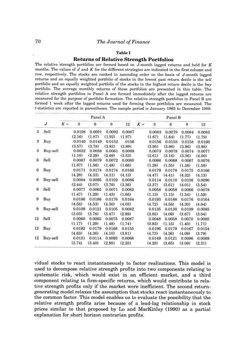
70 The Journal of Finance Table I Returns of Relative Strength Portfolios The relative 'strength portfolios are formed based on J-month lagged returns and held for K months.The values of J and K for the different strategies are indicated in the first column and row,respectively.The stocks are ranked in ascending order on the basis of J-month lagged returns and an equally weighted portfolio of stocks in the lowest past return decile is the sell portfolio and an equally weighted portfolio of the stocks in the highest return decile is the buy portfolio.The average monthly returns of these portfolios are presented in this table.The relative strength portfolios in Panel A are formed immediately after the lagged returns are measured for the purpose of portfolio formation.The relative strength portfolios in Panel B are formed 1 week after the lagged returns used for forming these portfolios are measured.The t-statistics are reported in parentheses.The sample period is January 1965 to December 1989. Panel A Panel B J K= 6 9 12 K- 6 9 12 3 Sell 0.01080.00910.00920.0087 0.00830.00790.0084 0.0083 (2.16) (1.87)(1.92) (1.87) (1.67) (1.64) (1.77) (1.79) 3 Buy 0.01400.01490.0152 .0156 0.0156 0.01580.0158 0.0160 (3.57) (3.78) (3.83) (3.89) (3.95) (3.98) (3.96) (3.98) 3 Buy-sell 0.00320.0058 0.00610.0069 0.00730.00780.00740.0077 (1.10) (2.29) (2.69) (3.53) (2.61) (3.16) (3.36) (4.00) 6 Sell 0.00870.00790.0072 0.0080 0.00660.00680.0067 0.0076 (1.67) (1.56)(1.48) (1.66) (1.28) (1.35) (1.38) (1.58) 6 Buy 0.01710.0174 0.0174 0.0166 0.01790.0178 0.0175 0.0166 (4.28) (4.33) (4.31) (4.13) (4.47) (4.41)(4.32) (4.13) 6 Buy-sell 0.00840.00950.01020.0086 0.01140.01100.0108 0.0090 (2.44) (3.07) (3.76) (3.36) (3.37) (3.61) (4.01) (3.54) 9 Sell 0.00770.0065 0.0071 0.0082 0.00580.0058 0.0066 0.0078 (1.47) (1.29) (1.43) (1.66) (1.13) (1.15)(1.34) (1.59) 9 Buy 0.01860.01860.0176 0.0164 0.01930.0188 0.01760.0164 (4.56) (4.53) (4.30) (4.03) (4.72) (4.56) (4.30) (4.04) 9 Buy-sell 0.0109 0.0121 0.0105 0.0082 0.0135 0.0130 0.0109 0.0085 (3.03) (3.78) (3.47) (2.89) (3.85) (4.09) (3.67) (3.04) 12 Sell 0.00600.00650.00750.0087 0.00480.00580.00700.0085 (1.17) (1.29) (1.48) (1.74) (0.93) (1.15) (1.40) (1.71) 12 Buy 0.01920.0179 0.01680.0155 0.01960.01790.0167 0.0154 (4.63)(4.36) (4.10) (3.81) (4.73) (4.36) (4.09) (3.79) 12 Buy-sell 0.01310.01140.00930.0068 0.01490.01210.0096 0.0069 (3.74) (3.40) (2.95) (2.25) (4.28) (3.65) (3.09) (2.31) vidual stocks to react instantaneously to factor realizations.This model is used to decompose relative strength profits into two components relating to systematic risk,which would exist in an efficient market,and a third component relating to firm-specific returns,which would contribute to rela- tive strength profits only if the market were inefficient.The second return- generating model relaxes the assumption that stocks react instantaneously to the common factor.This model enables us to evaluate the possibility that the relative strength profits arise because of a lead-lag relationship in stock prices similar to that proposed by Lo and MacKinlay (1990)as a partial explanation for short horizon contrarian profits
Returns to Buying Winners and Selling Losers 71 A.A Simple One-Factor Model Consider the following one-factor model describing stock returns: rit ui+bift+eu, E(f)=0 E(e)-0 (1) Cov(eit,f:)=0, i Cov(eit,eit-1)=0, i卡j where u is the unconditional expected return on security i,ri is the return on security i,f is the unconditional unexpected return on a factor- mimicking portfolio,ei:is the firm-specific component of return at time t,and 6,is the factor sensitivity of security i.For the 6-month/6-month strategy that we consider in the rest of this paper the length of a period is 6 months. The superior performance of the relative strength strategies documented in the last section implies that stocks that generate higher than average returns in one period also generate higher than average returns in the period that follows.In other words,these results imply that: E(r:-.lr4-1-7-1>0)>0 and E(rt-Trt-1-7-10. (2) The above cross-sectional covariance equals the expected profits from the zero-cost contrarian trading strategy examined by Lehmann(1990)and Lo and MacKinlay(1990)that weights stocks by their past returns less the past equally weighted index returns.This weighted relative strength strategy (WRSS)is closely related to our strategy.The WRSS yields a profit of 4.5% per dollar long semiannually(t-statistic =2.99)and the correlation between the returns of this strategy and that of the trading strategy examined in the last section is 0.95.The equally weighted decile portfolios are used in most of our empirical tests since they provide relatively more information than the WRSS.However,as the following analysis demonstrates,the closely related WRSS provides a tractable framework for analytically examining the sources of relative strength profits and evaluating the relative importance of each of these sources. 'Our analysis in this subsection is similar to that in Jegadeesh(1987)and Lo and MacKinlay (1990)
72 The Journal of Finance Given the one-factor model defined in (1),the WRSS profits given in expression(2)can be decomposed into the following three terms: E((rit -F)(rit-1-F:-1)}=g2+oCov(f,f:-1) Covi(eit,eit-1), (3) where o2 and are the cross-sectional variances of expected returns and factor sensitivities respectively. The above decomposition suggests three potential sources of the relative strength profits.The first term in this expression is the cross-sectional dispersion in expected returns.Intuitively,since realized returns contain a component related to expected returns,securities that experience relatively high returns in one period can be expected to have higher than average returns in the following period.The second term is related to the potential to time the factor.If the factor portfolio returns exhibit positive serial correla- tion,the relative strength strategy will tend to pick stocks with high b's when the conditional expectation of the factor portfolio return is high.As the above expression demonstrates,the extent to which relative strength strate- gies generate profits because of the serial correlation of the factor portfolio return is a function of the cross-sectional variance of the b's.The last term in the above expression is the average serial covariance of the idiosyncratic components of security returns. To assess whether the existence of relative strength profits imply market inefficiency,it is important to identify the sources of the profits.If the profits are due to either the first or the second term in expression(3)they may be attributed to compensation for bearing systematic risk and need not be an indication of market inefficiency.However,if the superior performance of the relative strength strategies is due to the third term,then the results would suggest market inefficiency. B.The Average Size and Beta of Relative Strength Portfolios This subsection considers the possibility that relative strength strategies systematically pick high-risk stocks and benefit from the first term in expres- sion (3).Table II reports estimates of the two most common indicators of systematic risk,the post-ranking betas of the ten 6-month/6-month relative strength portfolios and the average capitalizations of the stocks in these portfolios.The betas of the extreme past returns portfolios are higher than the average beta for the full sample.In addition,since the beta of the portfolio of past losers is higher than the beta of the portfolio of past winners, the beta of the zero-cost winners minus losers portfolio is negative.The average capitalizations of the stocks in the different portfolios show that the highest and the lowest past returns portfolios consist of smaller than average stocks,with the stocks in the losers portfolios being smaller than the stocks in the winners portfolio.This evidence suggests that the observed relative strength profits are not due to the first source of profits in expression (3)
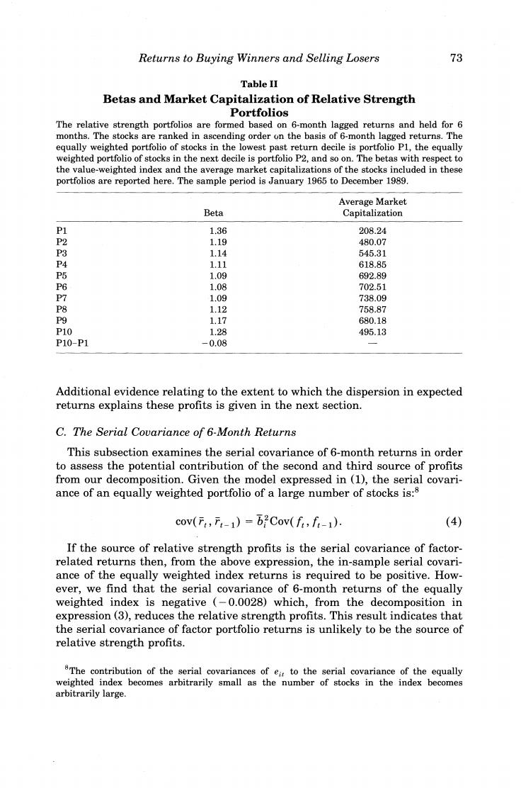
Returns to Buying Winners and Selling Losers 73 Table II Betas and Market Capitalization of Relative Strength Portfolios The relative strength portfolios are formed based on 6-month lagged returns and held for 6 months.The stocks are ranked in ascending order on the basis of 6-month lagged returns.The equally weighted portfolio of stocks in the lowest past return decile is portfolio Pl,the equally weighted portfolio of stocks in the next decile is portfolio P2,and so on.The betas with respect to the value-weighted index and the average market capitalizations of the stocks included in these portfolios are reported here.The sample period is January 1965 to December 1989. Average Market Beta Capitalization P1 1.36 208.24 P2 1.19 480.07 P3 1.14 545.31 P4 1.11 618.85 P5 1.09 692.89 P6 1.08 702.51 P7 1.09 738.09 P8 1.12 758.87 P9 1.17 680.18 P10 1.28 495.13 P10-P1 -0.08 Additional evidence relating to the extent to which the dispersion in expected returns explains these profits is given in the next section. C.The Serial Covariance of 6-Month Returns This subsection examines the serial covariance of 6-month returns in order to assess the potential contribution of the second and third source of profits from our decomposition.Given the model expressed in (1),the serial covari- ance of an equally weighted portfolio of a large number of stocks is:8 cov(,1)=b2Cov(f,f-1). (4) If the source of relative strength profits is the serial covariance of factor- related returns then,from the above expression,the in-sample serial covari- ance of the equally weighted index returns is required to be positive.How- ever,we find that the serial covariance of 6-month returns of the equally weighted index is negative (-0.0028)which,from the decomposition in expression(3),reduces the relative strength profits.This result indicates that the serial covariance of factor portfolio returns is unlikely to be the source of relative strength profits. 8The contribution of the serial covariances of eit to the serial covariance of the equally weighted index becomes arbitrarily small as the number of stocks in the index becomes arbitrarily large