CHAPTER TEN The IS-LM Model macroeconomics N.Gregory Mankiw College of Management,HUST
macroeconomics N. Gregory Mankiw CHAPTER TEN The IS-LM Model macro College of Management, HUST
In this chapter you will learn the IS curve,and its relation to the Keynesian Cross the Loanable Funds model the LM curve,and its relation to the Theory of Liquidity Preference how the IS-LM model determines income and the interest rate in the short run when P is fixed CHAPTER 10 Aggregate Demand I slide 1
CHAPTER 10 Aggregate Demand I slide 1 In this chapter you will learn ▪ the IS curve, and its relation to – the Keynesian Cross – the Loanable Funds model ▪ the LM curve, and its relation to – the Theory of Liquidity Preference ▪ how the IS-LM model determines income and the interest rate in the short run when P is fixed
Content 1.The Keynesian Cross 2.Fiscal policy and the multiplier 3.The IS curve 4.The Theory of Liquidity Preference 5.The LM curve 6.IS-LM model 7.Chapter summary CHAPTER 10 Aggregate Demand I slide 2
CHAPTER 10 Aggregate Demand I slide 2 Content 1. The Keynesian Cross 2. Fiscal policy and the multiplier 3. The IS curve 4. The Theory of Liquidity Preference 5. The LM curve 6. IS-LM model 7. Chapter summary
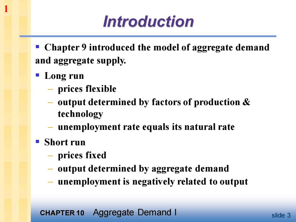
1 Introduction Chapter 9 introduced the model of aggregate demand and aggregate supply. ■Long run prices flexible 一 output determined by factors of production technology 一 unemployment rate equals its natural rate ▣Short run -prices fixed output determined by aggregate demand unemployment is negatively related to output CHAPTER 10 Aggregate Demand I slide 3
CHAPTER 10 Aggregate Demand I slide 3 Introduction ▪ Chapter 9 introduced the model of aggregate demand and aggregate supply. ▪ Long run – prices flexible – output determined by factors of production & technology – unemployment rate equals its natural rate ▪ Short run – prices fixed – output determined by aggregate demand – unemployment is negatively related to output 1
Introduction This chapter develops the IS-LM model,the theory that yields the aggregate demand curve. We focus on the short run and assume the price level is fixed. CHAPTER 10 Aggregate Demand I slide 4
CHAPTER 10 Aggregate Demand I slide 4 Introduction ▪ This chapter develops the IS-LM model, the theory that yields the aggregate demand curve. ▪ We focus on the short run and assume the price level is fixed. 1
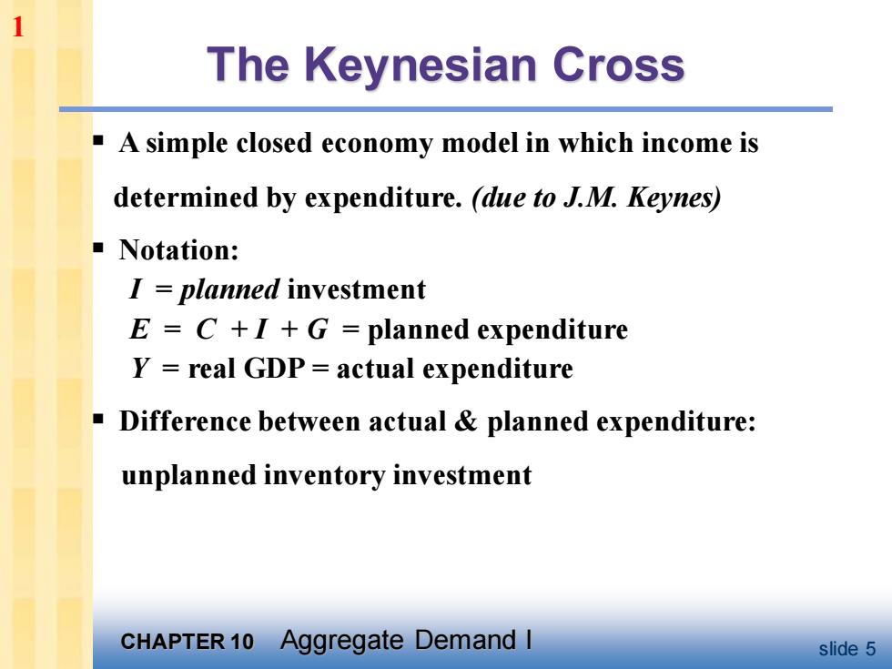
1 The Keynesian Cross A simple closed economy model in which income is determined by expenditure.(due to J.M.Keynes) ▣Notation: I planned investment E=C+I+G planned expenditure Y=real GDP=actual expenditure Difference between actual planned expenditure: unplanned inventory investment CHAPTER 10 Aggregate Demand I slide 5
CHAPTER 10 Aggregate Demand I slide 5 The Keynesian Cross ▪ A simple closed economy model in which income is determined by expenditure. (due to J.M. Keynes) ▪ Notation: I = planned investment E = C + I + G = planned expenditure Y = real GDP = actual expenditure ▪ Difference between actual & planned expenditure: unplanned inventory investment 1
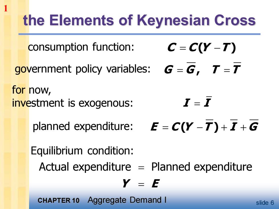
1 the Elements of Keynesian Cross consumption function: C=C(Y-T) government policy variables:G=G,T= for now, investment is exogenous: T-T planned expenditure:E=C(Y-T)++G Equilibrium condition: Actual expenditure =Planned expenditure Y=E CHAPTER 10 Aggregate Demand I slide 6
CHAPTER 10 Aggregate Demand I slide 6 the Elements of Keynesian Cross C C Y T = − ( ) I I = G G T T = = , E C Y T I G = − + + ( ) Actual expenditure Planned expenditure Y E = = consumption function: for now, investment is exogenous: planned expenditure: Equilibrium condition: government policy variables: 1
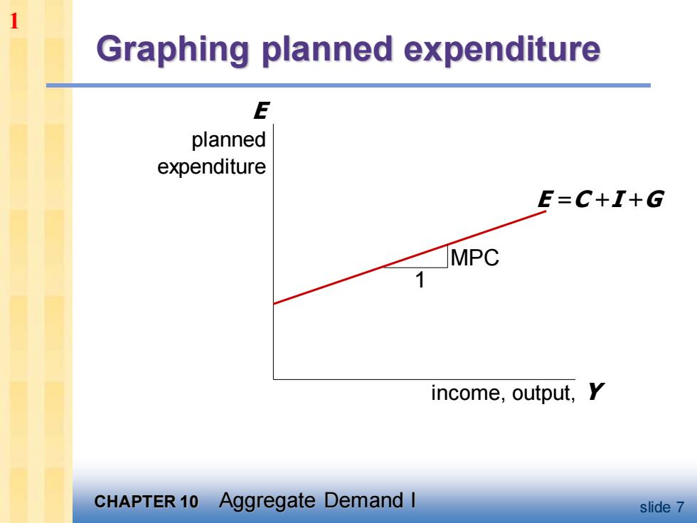
1 Graphing planned expenditure E planned expenditure E=C+I+G MPC income,output,Y CHAPTER 10 Aggregate Demand I slide 7
CHAPTER 10 Aggregate Demand I slide 7 Graphing planned expenditure income, output, Y E planned expenditure E =C +I +G MPC 1 1
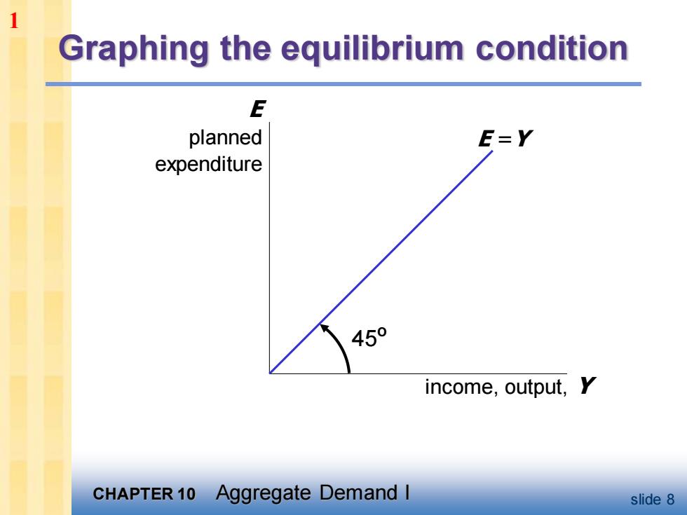
1 Graphing the equilibrium condition E planned E=Y expenditure 450 income,output,Y CHAPTER 10 Aggregate Demand I slide 8
CHAPTER 10 Aggregate Demand I slide 8 Graphing the equilibrium condition income, output, Y E planned expenditure E =Y 45º 1
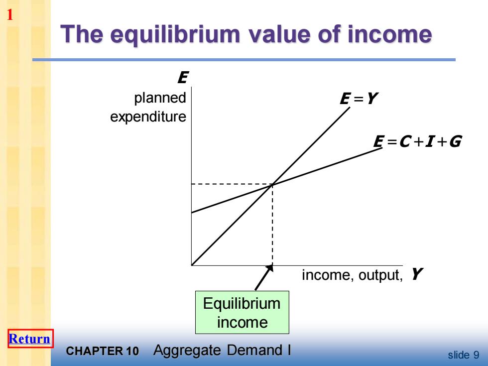
1 The equilibrium value of income E planned E=Y expenditure E=C+I+G income,output,Y Equilibrium income Return CHAPTER 10 Aggregate Demand I slide 9
CHAPTER 10 Aggregate Demand I slide 9 The equilibrium value of income income, output, Y E planned expenditure E =Y E =C +I +G Equilibrium income 1 Return