上海交通大学：《传热传质学 Heat and Mass Transfer》教学资源（课程讲义）Lecture Notes_hch6 INTRODUCTION（2/2）

Boundary Layer Similarity Parameters The boundary layer equations(velocity,mass, energy continuity)represent low speed,forced convection flow. Advection terms on the left side and diffusion terms on the right side of each equation, such as: Advection TT Diffusion W- Ox dy 0y2 Non-dimensionalize the equations by setting ond y where L is characteristic length of the surface and v-y where V is the freestream velocity (U) and T-T and P=p/pv2 T-T

Boundary Layer Similarity Parameters • The boundary layer equations (velocity, mass, energy continuity) represent low speed, forced convection flow. • Advection terms on the left side and diffusion terms on the right side of each equation, such as: Advection Diffusion • Non-dimensionalize the equations by setting: * s * 2 and / T T -T and where V is the freestream velocity ( ) where L is characteristic length of the surface P p V T T U V v and v V u u L y and y L x x s                2 2 y T y T v x T u         

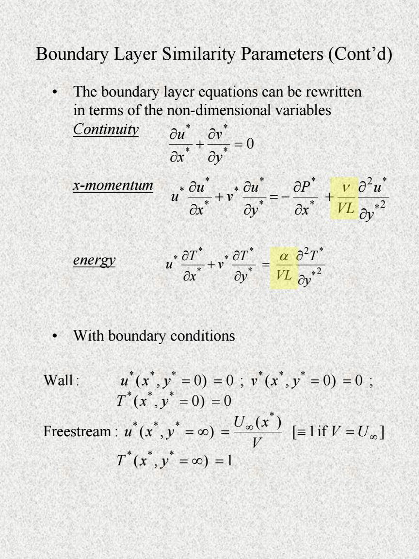
Boundary Layer Similarity Parameters(Cont'd) The boundary layer equations can be rewritten in terms of the non-dimensional variables Continuity ou,0* * =0 x-momentum aP O2u' +v Ox" ov" Ox L *2 a energy tv'o *dT* o2T u 元0y2 With boundary conditions Wall u(x,y=0)=0;v*(x,y=0)=0; T(x,y=0)=0 Frcestream:)U)if-U] T(x,y*=o)=1

Boundary Layer Similarity Parameters (Cont’d) • The boundary layer equations can be rewritten in terms of the non-dimensional variables Continuity x-momentum energy • With boundary conditions 0 * * * *       y v x u 2 * 2 * * * * * * * * * y u x VL P y u v x u u              2 * 2 * * * * * * * y T y VL T v x T u          ( , ) 1 [ 1if ] ( ) Freestream : ( , ) ( , 0) 0 Wall : ( , 0) 0 ; ( , 0) 0 ; * * * * * * * * * * * * * * * *                 T x y V U V U x u x y T x y u x y v x y

Boundary Layer Similarity Parameters(Cont'd) From the non-dimensionalized boundary layer equations,dimensionless groups can be seen Reynolds Prandtl Substituting gives the boundary layer equations: Continuity: ou'Ov" =0 * ou'ou ap* 1a2u* x-momentum: u +v Ox a" ReL oy Energy: aT,*∂T*1 02T dy" ReLPry2

Boundary Layer Similarity Parameters (Cont’d) • From the non-dimensionalized boundary layer equations, dimensionless groups can be seen Reynolds # Prandtl # Substituting gives the boundary layer equations:  VL Re L  0 * * * *       y v x u 2 * 2 * * * * * * * * * Re 1 y u x P y u v x u u L             Re Pr 1 2 * 2 * * * * * * * y T y T v x T u L          Continuity: x-momentum: Energy:   P r 

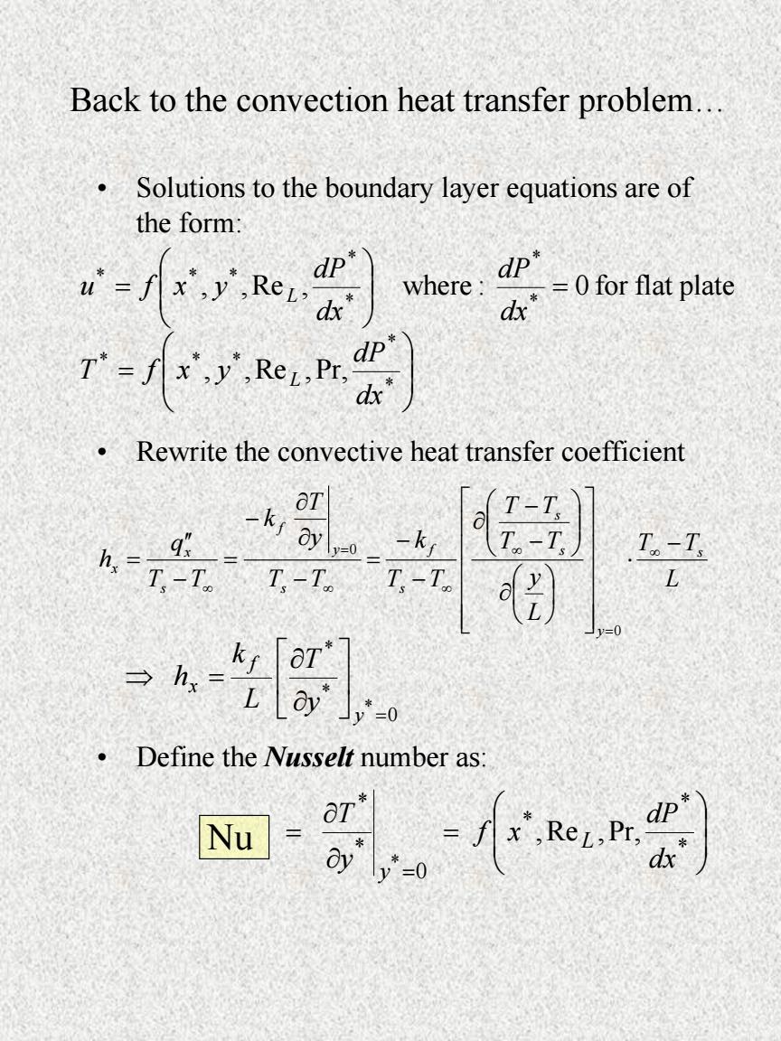
Back to the convection heat transfer problem... Solutions to the boundary layer equations are of the form: =,） dP" where: =0 for flat plate x* -小器 .Rewrite the convective heat transfer coefficient t 一k 6 T-T -ki h, 9 T。-I T,-T. T-T。 T-T. L kr 「a Define the Nusselt number as: Nu .o

Back to the convection heat transfer problem… • Solutions to the boundary layer equations are of the form: • Rewrite the convective heat transfer coefficient • Define the Nusselt number as:                * * * * * * * * * * * * , ,Re ,Pr, , ,Re , where : 0 for flat plate dx dP T f x y dx dP dx dP u f x y L L L T T L y T T T T T T k T T y T k T T q h s y s s s f s y f s x x                                         0 0 0 * * *           y f x y T L k h            * * * 0 * * ,Re ,Pr, * dx dP f x y T L y Nu

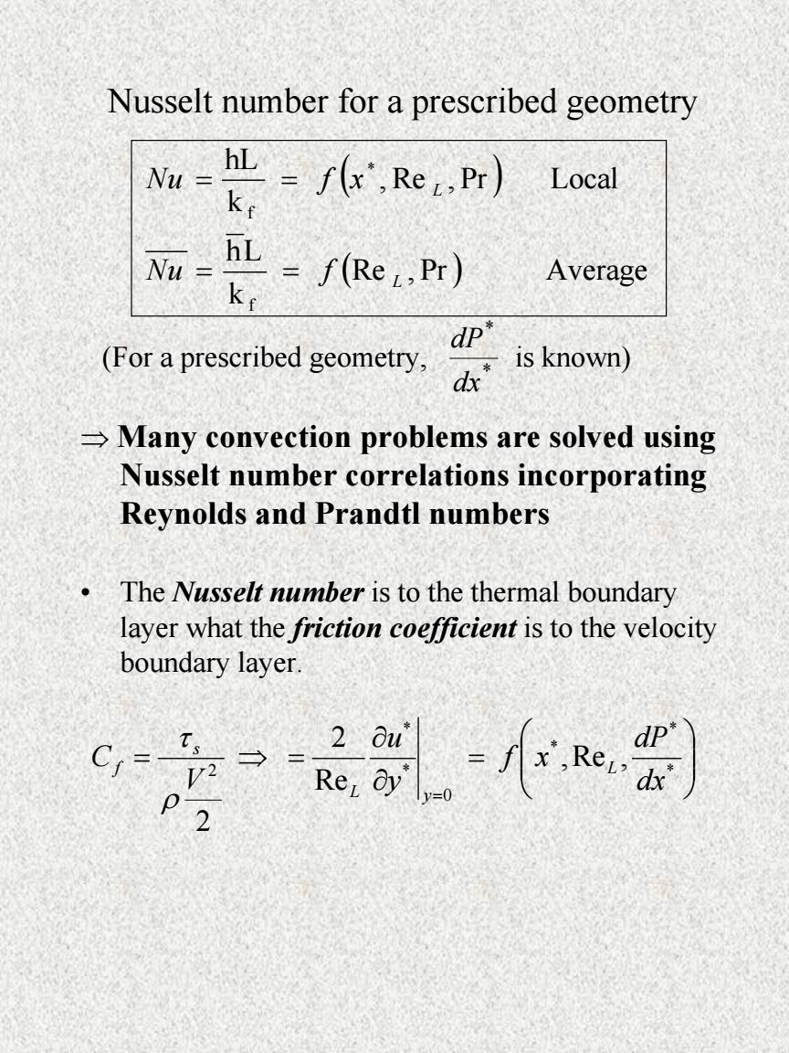
Nusselt number for a prescribed geometry Nu= -=f(x'.Rec.Pr) Local Nu= _=f(Re.Pr) Average dp" (For a prescribed geometry, is known) dx Many convection problems are solved using Nusselt number correlations incorporating Reynolds and Prandtl numbers The Nusselt number is to the thermal boundary layer what the friction coefficient is to the velocity boundary layer. CI= 2 ou v2 → Re,dy" =0 2

Nusselt number for a prescribed geometry (For a prescribed geometry, is known)  Many convection problems are solved using Nusselt number correlations incorporating Reynolds and Prandtl numbers • The Nusselt number is to the thermal boundary layer what the friction coef icient is to the velocity boundary layer.   Re , Pr  Average k hL , Re , Pr Local k hL f * f L L Nu f Nu f x     * * dx dP              * * * 0 * * 2 ,Re , Re 2 2 dx dP f x y u V C L L y s f  

Heat transfer coefficient,simple example Given: Air at 20C flowing over heated flat plate at 100C.Experimental measurements of temperatures at various distances from the surface are as shown Experimental measurements Experiinental measurements 2 mm 1.2 mm =66.7 mm Air now Surface of plate 20 50 100C .Find:convective heat transfer coefficient,h

Heat transfer coefficient, simple example • Given: Air at 20ºC flowing over heated flat plate at 100ºC. Experimental measurements of temperatures at various distances from the surface are as shown • Find: convective heat transfer coefficient, h Experimental measurements

Heat transfer coefficient,simple example ·Solution: OT Rccall that h is computed by Ts-To From Table A-4 in Appendix,at a mean fluid temperature 7n7。+7 2 (average of free-stream and surface temperatures) Tm=(20+100)/2=60°C the air conductivity,k is=0.028 W/m-K ● Temperature gradient at the plate surface from experimental data is-66.7 K/mm =-66,700 K/m So,convective heat transfer coefficient is: h、 -0.028×(-66700) 80 W =23.345 m2K

Heat transfer coefficient, simple example • Solution: Recall that h is computed by • From Table A-4 in Appendix, at a mean fluid temperature (average of free-stream and surface temperatures) the air conductivity, k is  0.028 W/m-K • Temperature gradient at the plate surface from experimental data is -66.7 K/mm = -66,700 K/m • So, convective heat transfer coefficient is: 0        T T y T k h s y f x m K W 23.345 80 - 0.028 ( 66700) 2    h  2 m T Ts T    T C  m  (20 100) 2  60

SUMMARY General boundary layer equations Ou av dx dy -0 u Bu 1 aP Ou u- +V =0 ay pox dy2 ay [=a 2T +V- Ox C 2 Nusselt number for heat transfer coefficient in the thermal boundary layer Nu= =f(.ReL.P) K Local Nu= L=f(ReL.Pr) Average Many convection problems are solved using Nusselt number correlations incorporating Reynolds and Prandtl numbers

• General boundary layer equations • Nusselt number for heat transfer coefficient in the thermal boundary layer • Many convection problems are solved using Nusselt number correlations incorporating Reynolds and Prandtl numbers. SUMMARY  0      y v x u 2 2 1 y u x P y u v x u u                0   y P 2 2 2                  y u y c T y T v x T u p     Re ,Pr Average ,Re ,Pr Local * L f L f f k h L Nu f x k h L Nu    

Momentum and Heat Transfer Analogy IF WE CAN PUT A MAN YOUR FLAWED ANALO- MAYBE YOU SHOULD ON THE MOON,WE CAN GY ONLY SHOWS THAT CALL OTHER PEOPLE BUILD A COMPUTER OTHER PEOPLE CAN AND ASK HOW THEY MADE ENTIRELY OF DO OTHER THINGS. DO IT. RECYCLED PAPER. MAYBE THEY USE GOOD ANALOGIES Copyright 3 2002 United Feature Syndicate,Inc

Momentum and Heat Transfer Analogy

Momentum and Heat Transfer Analogy Where we've been...... Development of convective transport of heat transfer equations Where we're going: Momentum and heat transfer(Reynolds)analogy

Momentum and Heat Transfer Analogy Where we’ve been …… • Development of convective transport of heat transfer equations Where we’re going: • Momentum and heat transfer (Reynolds) analogy