9 Inference Uncertainty and it doesn't rain and my tires remain intact etc etc.' noisy sensors(KCBS traffic reports) Independence and Syntax and Semantics bility (road state,other drivers'plans,etc. Uncertainty Outline UNCERTAINT maki !. Which action to choose? gets me there on timel me there on time Suppose I belive the fallowing: Making decisions under uncertainty (Anabgous to logical entailment status not truth.) Default ar nonmonotonic logic: Probability Issues:Problems with combination,e.g..Sprinler causes Rain?? Assume my car does not have a flat tire Methods for handling uncertainty
Uncertainty Chapter 13 Chapter 13 1 Outline ♦ Uncertainty ♦ Probability ♦ Syntax and Semantics ♦ Inference ♦ Independence and Bayes’ Rule Chapter 13 2 Uncertainty Let action At = leave for airport t minutes before flight Will At get me there on time? Problems: 1) partial observability (road state, other drivers’ plans, etc.) 2) noisy sensors (KCBS traffic reports) 3) uncertainty in action outcomes (flat tire, etc.) 4) immense complexity of modelling and predicting traffic Hence a purely logical approach either 1) risks falsehood: “A25 will get me there on time” or 2) leads to conclusions that are too weak for decision making: “A25 will get me there on time if there’s no accident on the bridge and it doesn’t rain and my tires remain intact etc etc.” A( 1440 might reasonably be said to get me there on time but I’d have to stay overnight in the airport . . .) Chapter 13 3 Methods for handling uncertainty Default or nonmonotonic logic: Assume my car does not have a flat tire Assume A25 works unless contradicted by evidence Issues: What assumptions are reasonable? How to handle contradiction? Rules with fudge factors: A25 7→0.3 AtAirportOnTime Sprinkler 7→0.99 WetGrass WetGrass 7→0.7 Rain Issues: Problems with combination, e.g., Sprinkler causes Rain?? Probability Given the available evidence, A25 will get me there on time with probability 0.04 Mahaviracarya (9th C.), Cardamo (1565) theory of gambling (Fuzzy logic handles degree of truth NOT uncertainty e.g., WetGrass is true to degree 0.2) Chapter 13 4 Probability Probabilistic assertions summarize effects of laziness: failure to enumerate exceptions, qualifications, etc. ignorance: lack of relevant facts, initial conditions, etc. Subjective or Bayesian probability: Probabilities relate propositions to one’s own state of knowledge e.g., P(A25|no reported accidents) = 0.06 These are not claims of a “probabilistic tendency” in the current situation (but might be learned from past experience of similar situations) Probabilities of propositions change with new evidence: e.g., P(A25|no reported accidents, 5 a.m.) = 0.15 (Analogous to logical entailment status KB |= α, not truth.) Chapter 13 5 Making decisions under uncertainty Suppose I believe the following: P(A25 gets me there on time| . . .) = 0.04 P(A90 gets me there on time| . . .) = 0.70 P(A120 gets me there on time| . . .) = 0.95 P(A1440 gets me there on time| . . .) = 0.9999 Which action to choose? Depends on my preferences for missing flight vs. airport cuisine, etc. Utility theory is used to represent and infer preferences Decision theory = utility theory + probability theory Chapter 13 6
event=set of sam Given Bodean adom event aset of sample variables A and B: ible rolls of a die. Begin with a set 1-the sample space FPiooampnalermg Often in Al applications,the sample points are ded event a=points where A(w)=true and Bw)=true points where Aw)=fr Propositions e.g.P(Odd=trwe)=P(1)+P(3)+P(5)=1/6+1+1/6=1/2 Random variables Eg..P(die roll <)=P(1)+P(2)+P(3)1/6+1/6+1/6=1/2 Probability basics Joint probability distribution for a set of r.vs gives the Prior probability e.g.Temp=21.6;aso allow,e.g..Temp <22.0 an random variables Syntax for propositions E.g.P(av)=P(a)+p()-P(a) The definitiom imply that certain gically related events must have related Why use probability?
Probability basics Begin with a set Ω—the sample space e.g., 6 possible rolls of a die. ω ∈ Ω is a sample point/possible world/atomic event A probability space or probability model is a sample space with an assignment P(ω) for every ω ∈ Ω s.t. 0 ≤ P(ω) ≤ 1 ΣωP(ω) = 1 e.g., P(1) = P(2) = P(3) = P(4) = P(5) = P(6) = 1/6. An event A is any subset of Ω P(A) = Σ{ω∈A}P(ω) E.g., P(die roll A B True A B de Finetti (1931): an agent who bets according to probabilities that violate these axioms can be forced to bet so as to lose money regardless of outcome. Chapter 13 10 Syntax for propositions Propositional or Boolean random variables e.g., Cavity (do I have a cavity?) Cavity = true is a proposition, also written cavity Discrete random variables (finite or infinite) e.g., Weather is one of hsunny, rain, cloudy, snowi Weather = rain is a proposition Values must be exhaustive and mutually exclusive Continuous random variables (bounded or unbounded) e.g., Temp = 21.6; also allow, e.g., Temp < 22.0. Arbitrary Boolean combinations of basic propositions Chapter 13 11 Prior probability Prior or unconditional probabilities of propositions e.g., P(Cavity = true) = 0.1 and P(Weather = sunny) = 0.72 correspond to belief prior to arrival of any (new) evidence Probability distribution gives values for all possible assignments: P(Weather) = h0.72, 0.1, 0.08, 0.1i (normalized, i.e., sums to 1) Joint probability distribution for a set of r.v.s gives the probability of every atomic event on those r.v.s (i.e., every sample point) P(Weather, Cavity) = a 4 × 2 matrix of values: Weather = sunny rain cloudy snow Cavity = true 0.144 0.02 0.016 0.02 Cavity = false 0.576 0.08 0.064 0.08 Every question about a domain can be answered by the joint distribution because every event is a sum of sample points Chapter 13 12
This kind of inference,sanctioned by domain knowldge,is crucial If we know more,is ako given,then we have P[)2-element vector of 2-clement vectors) 5100r00m450Ta14510010m NOT f then chance of onrity" 异 Conditional probability Gaussian density Probability for continuous variables P(toot)=(.108+1+0.(64=0.2 cavin .016 with the jointdist Definition of conditional probability .064.144/.576 012 072.009 catch catch catch Inference by enumeration o675.441·460:6t e .i08.12.072.00 catchcatch catch Inference by enumeration (View as a4x 2 set of equations,not matrix mult.) Conditional probability
Probability for continuous variables Express distribution as a parameterized function of value: P(X = x) = U[18, 26](x) = uniform density between 18 and 26 0.125 dx 18 26 Here P is a density; integrates to 1. P(X = 20.5) = 0.125 really means dx lim→0 P(20.5 ≤ X ≤ 20.5 + dx)/dx = 0.125 Chapter 13 13 Gaussian density P(x) = 1 √ 2πσ e −(x−µ) 2/2σ 2 0 Chapter 13 14 Conditional probability Conditional or posterior probabilities e.g., P(cavity|toothache) = 0.8 i.e., given that toothache is all I know NOT “if toothache then 80% chance of cavity” (Notation for conditional distributions: P(Cavity|Toothache) = 2-element vector of 2-element vectors) If we know more, e.g., cavity is also given, then we have P(cavity|toothache, cavity) = 1 Note: the less specific belief remains valid after more evidence arrives, but is not always useful New evidence may be irrelevant, allowing simplification, e.g., P(cavity|toothache, 49ersWin) = P(cavity|toothache) = 0.8 This kind of inference, sanctioned by domain knowledge, is crucial Chapter 13 15 Conditional probability Definition of conditional probability: P(a|b) = P(a ∧ b) P(b) if P(b) 6= 0 Product rule gives an alternative formulation: P(a ∧ b) = P(a|b)P(b) = P(b|a)P(a) A general version holds for whole distributions, e.g., P(Weather, Cavity) = P(Weather|Cavity)P(Cavity) (View as a 4 × 2 set of equations, not matrix mult.) Chain rule is derived by successive application of product rule: P(X1, . . . , Xn) = P(X1, . . . , Xn−1) P(Xn|X1, . . . , Xn−1) = P(X1, . . . , Xn−2) P(Xn1 |X1, . . . , Xn−2) P(Xn|X1, . . . , Xn−1) = . . . = Πi n = 1P(Xi |X1, . . . , Xi−1) Chapter 13 16 Inference by enumeration Start with the joint distribution: cavity L toothache cavity catch catch L toothache L catch catch L .108 .012 .016 .064 .144 .072 .576 .008 For any proposition φ, sum the atomic events where it is true: P(φ) = Σω:ω|=φP(ω) Chapter 13 17 Inference by enumeration Start with the joint distribution: cavity L toothache cavity catch catch L toothache L catch catch L .108 .012 .016 .064 .144 .072 .576 .008 For any proposition φ, sum the atomic events where it is true: P(φ) = Σω:ω|=φP(ω) P(toothache) = 0.108 + 0.012 + 0.016 + 0.064 = 0.2 Chapter 13 18
=P(Cavilu,toothache.catch)+P[Cavitu,tod.catch' Start with the joint distrbution 108 .012 -108.m2 .016.064 .10.12 .144.57 he/.94.144.76 .72.009 Inference by enumeration .144-57m .272.008 Inference by enumeration independence but rare the poster da P(Toothache,Carity.Cateh)has-1-7 independent entries Conditional independence Independence Inference by enumeration,contd
Inference by enumeration Start with the joint distribution: cavity L toothache cavity catch catch L toothache L catch catch L .108 .012 .016 .064 .144 .072 .576 .008 For any proposition φ, sum the atomic events where it is true: P(φ) = Σω:ω|=φP(ω) P(cavity∨toothache) = 0.108+0.012+0.072+0.008+0.016+0.064 = 0.28 Chapter 13 19 Inference by enumeration Start with the joint distribution: cavity L toothache cavity catch catch L toothache L catch catch L .108 .012 .016 .064 .144 .072 .576 .008 Can also compute conditional probabilities: P(¬cavity|toothache) = P(¬cavity ∧ toothache) P(toothache) = 0.016 + 0.064 0.108 + 0.012 + 0.016 + 0.064 = 0. Chapter 4 13 20 Normalization cavity L toothache cavity catch catch L toothache L catch catch L .108 .012 .016 .064 .144 .072 .576 .008 Denominator can be viewed as a normalization constant α P(Cavity|toothache) = α P(Cavity,toothache) = α [P(Cavity,toothache, catch) + P(Cavity,toothache,¬catch)] = α [h0.108, 0.016i + h0.012, 0.064i] = α h0.12, 0.08i = h0.6, 0.4i General idea: compute distribution on query variable by fixing evidence variables and summing over hidden variables Chapter 13 21 Inference by enumeration, contd. Let X be all the variables. Typically, we want the posterior joint distribution of the query variables Y given specific values e for the evidence variables E Let the hidden variables be H = X − Y − E Then the required summation of joint entries is done by summing out the hidden variables: P(Y|E = e) = αP(Y, E = e) = αΣhP(Y, E = e, H = h) The terms in the summation are joint entries because Y, E, and H together exhaust the set of random variables Obvious problems: 1) Worst-case time complexity O(d n ) where d is the largest arity 2) Space complexity O(d n ) to store the joint distribution 3) How to find the numbers for O(d n ) entries??? Chapter 13 22 Independence A and B are independent iff P(A|B) = P(A) or P(B|A) = P(B) or P(A, B) = P(A)P(B) Weather Toothache Catch Cavity decomposes into Weather Toothache Catch Cavity P(Toothache, Catch, Cavity, Weather) = P(Toothache, Catch, Cavity)P(Weather) 32 entries reduced to 12; for n independent biased coins, 2 n → n Absolute independence powerful but rare Dentistry is a large field with hundreds of variables, none of which are independent. What to do? Chapter 13 23 Conditional independence P(Toothache, Cavity, Catch) has 2 3 − 1 = 7 independent entries If I have a cavity, the probability that the probe catches in it doesn’t depend on whether I have a toothache: (1) P(catch|toothache, cavity) = P(catch|cavity) The same independence holds if I haven’t got a cavity: (2) P(catch|toothache,¬cavity) = P(catch|¬cavity) Catch is conditionally independent of Toothache given Cavity: P(Catch|Toothache, Cavity) = P(Catch|Cavity) Equivalent statements: P(Toothache|Catch, Cavity) = P(Toothache|Cavity) P(Toothache, Catch|Cavity) = P(Toothache|Cavity)P(Catch|Cavity) Chapter 13 24
Total number of parameters is liner in n P(Cause,Effech... Bayes'Rule and conditional independence P(s) Eg..let be meningitis,5 be stiff neck: =3 P(EJJeet) Product ruk P(a=(a=P()P(a) Bayes'Rule le.++1=5 independent numbers (equations 1 and 2 remove2) Write out full joint distribution using chain rule: Conditional independence contd. Grows exponentially with number of squares P(P..b-aP(Pia.unk nown.&nomn,b) For inference by enumeration,we hae Query is P(,b) Observations and query P(PP)=-1P()=02x08- erm:pits areplaced randomly probablitypersquare First term:1 if pits are adjacent to breezeotherwise (Do it this way to get P(fectCause).) Apply product rue:P(BB.B .P)P(P....Pu) The full joint distribution is P(P.P,B.B2,B21) Specifying the probability model P=true iffj]contains a pit Wumpus World
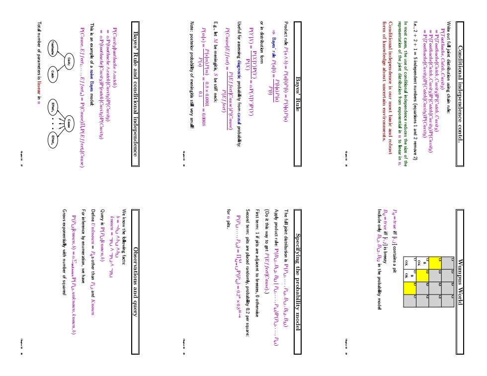
Conditional independence contd. Write out full joint distribution using chain rule: P(Toothache, Catch, Cavity) = P(Toothache|Catch, Cavity)P(Catch, Cavity) = P(Toothache|Catch, Cavity)P(Catch|Cavity)P(Cavity) = P(Toothache|Cavity)P(Catch|Cavity)P(Cavity) I.e., 2 + 2 + 1 = 5 independent numbers (equations 1 and 2 remove 2) In most cases, the use of conditional independence reduces the size of the representation of the joint distribution from exponential in n to linear in n. Conditional independence is our most basic and robust form of knowledge about uncertain environments. Chapter 13 25 Bayes’ Rule Product rule P(a ∧ b) = P(a|b)P(b) = P(b|a)P(a) ⇒ Bayes’ rule P(a|b) = P(b|a)P(a) P(b) or in distribution form P(Y |X) = P(X|Y )P(Y ) P(X) = αP(X|Y )P(Y ) Useful for assessing diagnostic probability from causal probability: P(Cause|Effect) = P(Effect|Cause)P(Cause) P(Effect) E.g., let M be meningitis, S be stiff neck: P(m|s) = P(s|m)P(m) P(s) = 0.8 × 0.0001 0.1 = 0.0008 Note: posterior probability of meningitis still very small! Chapter 13 26 Bayes’ Rule and conditional independence P(Cavity|toothache ∧ catch) = α P(toothache ∧ catch|Cavity)P(Cavity) = α P(toothache|Cavity)P(catch|Cavity)P(Cavity) This is an example of a naive Bayes model: P(Cause, Effect1, . . . , Effectn) = P(Cause)ΠiP(Effecti |Cause) Toothache Cavity Catch Cause Effect1 Effectn Total number of parameters is linear in n Chapter 13 27 Wumpus World OK 1,1 2,1 3,1 4,1 1,2 2,2 3,2 4,2 1,3 2,3 3,3 4,3 1,4 2,4 OK OK 3,4 4,4 B B Pij = true iff [i, j] contains a pit Bij = true iff [i, j] is breezy Include only B1,1, B1,2, B2,1 in the probability model Chapter 13 28 Specifying the probability model The full joint distribution is P(P1,1, . . . , P4,4, B1,1, B1,2, B2,1) Apply product rule: P(B1,1, B1,2, B2,1 | P1,1, . . . , P4,4)P(P1,1, . . . , P4,4) (Do it this way to get P(Effect|Cause).) First term: 1 if pits are adjacent to breezes, 0 otherwise Second term: pits are placed randomly, probability 0.2 per square: P(P1,1, . . . , P4,4) = Π 4,4 i,j = 1,1P(Pi,j) = 0.2 n × 0.8 16−n for n pits. Chapter 13 29 Observations and query We know the following facts: b = ¬b1,1 ∧ b1,2 ∧ b2,1 known = ¬p1,1 ∧ ¬p1,2 ∧ ¬p2,1 Query is P(P1,3|known, b) Define Unknown = Pijs other than P1,3 and Known For inference by enumeration, we have P(P1,3|known, b) = αΣunknownP(P1,3, unknown, known, b) Grows exponentially with number of squares! Chapter 13 30
P(,)0.8,0.14 P(Poien,5)o/0.2(0.04+0.16+0.1G),0.8(0.04+0.16) 08 x02-016 Using conditional independence contd. P(Pa)P(e,Pia.fringe)p(fringe) =Pnown,Fia.fringe)P(P(nonen)P(fringe)P( P(nown,Pia.fringeP(P,known,fringe,other) P(blinowen.Pi.fringe,other)P(P.known,fringe.other Using conditional independence contd. Manipulate queryinto a form where we can use this! Using conditional independence Independence and conditional independence provide the tools Fornontrivadomaiswe must find a way toreuce the joint size Queries can be answered by summing over atomic events Summary
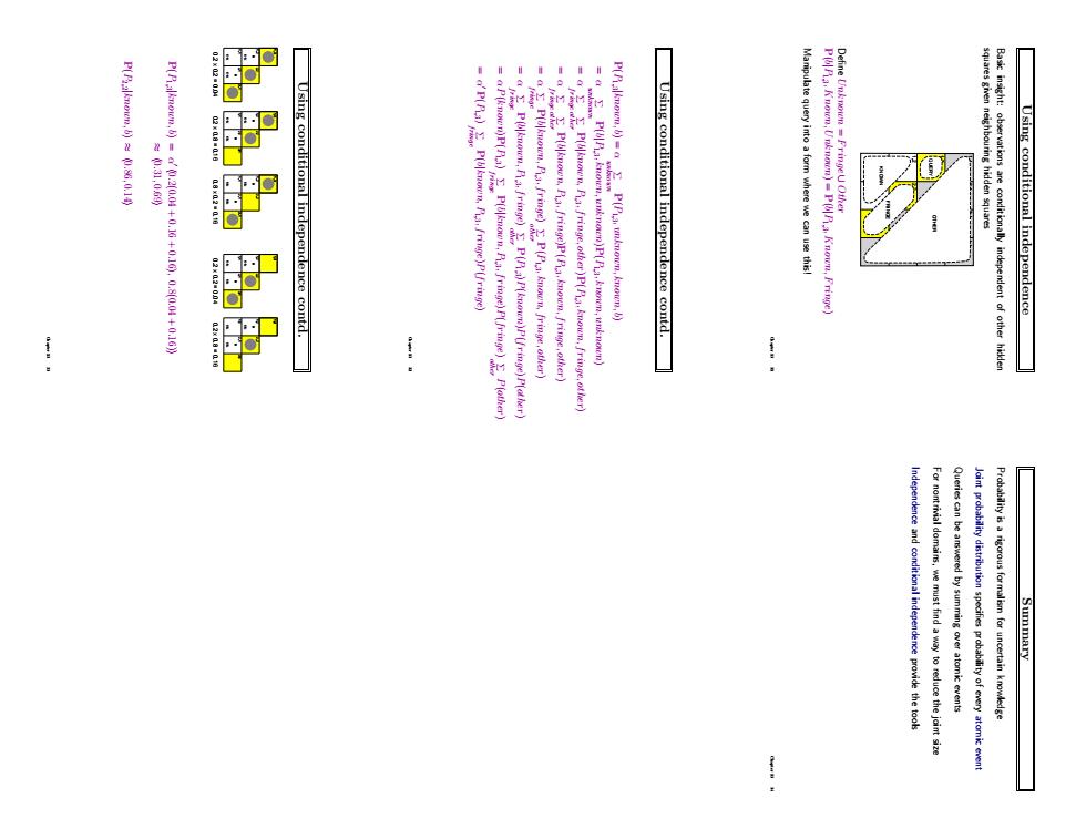
Using conditional independence Basic insight: observations are conditionally independent of other hidden squares given neighbouring hidden squares 1,1 2,1 3,1 4,1 1,2 2,2 3,2 4,2 1,3 2,3 3,3 4,3 1,4 2,4 3,4 4,4 KNOWN FRINGE QUERY OTHER Define Unknown = Fringe ∪ Other P(b|P1,3, Known,Unknown) = P(b|P1,3, Known, Fringe) Manipulate query into a form where we can use this! Chapter 13 31 Using conditional independence contd. P(P1,3|known, b) = α X unknown P(P1,3, unknown, known, b) = α X unknown P(b|P1,3, known, unknown)P(P1,3, known, unknown) = α X fringe X other P(b|known,P1,3, fringe, other)P(P1,3, known, fringe, other) = α X fringe X other P(b|known,P1,3, fringe)P(P1,3, known, fringe, other) = α X fringe P(b|known,P1,3, fringe) X other P(P1,3, known, fringe, other) = α X fringe P(b|known,P1,3, fringe) X other P(P1,3)P(known)P(fringe)P(other) = α P(known)P(P1,3) X fringe P(b|known,P1,3, fringe)P(fringe) X other P(other) = α 0 P(P1,3) X fringe P(b|known,P1,3, fringe)P(fringe) Chapter 13 32 Using conditional independence contd. OK 1,1 2,1 3,1 1,2 2,2 1,3 OK OK B B OK 1,1 2,1 3,1 1,2 2,2 1,3 OK OK B B OK 1,1 2,1 3,1 1,2 2,2 1,3 OK OK B B 0.2 x 0.2 = 0.04 0.2 x 0.8 = 0.16 0.8 x 0.2 = 0.16 OK 1,1 2,1 3,1 1,2 2,2 1,3 OK OK B B OK 1,1 2,1 3,1 1,2 2,2 1,3 OK OK B B 0.2 x 0.2 = 0.04 0.2 x 0.8 = 0.16 P(P1,3|known, b) = α 0 h0.2(0.04 + 0.16 + 0.16), 0.8(0.04 + 0.16)i ≈ h0.31, 0.69i P(P2,2|known, b) ≈ h0.86, 0.14i Chapter 13 33 Summary Probability is a rigorous formalism for uncertain knowledge Joint probability distribution specifies probability of every atomic event Queries can be answered by summing over atomic events For nontrivial domains, we must find a way to reduce the joint size Independence and conditional independence provide the tools Chapter 13 34