上游充通大¥ SHANGHAI JIAO TONG UNIVERSITY Chapter 3 Generalized performance characteristics of instruments by Yixin Ma 06/03/2013 2/88 Contents ·Introduction Static Characteristics(静态特性)& Static Calibration(静态标定) ·Dynamic Characteristics(动态特性)
Chapter 3 Generalized performance characteristics of instruments by Yixin Ma 06/03/2013 Contents • Introduction • Static Characteristics(静态特性) & Static Calibration (静态标定) • Dynamic Characteristics(动态特性) 2/88
3/88 3.1 Introduction Why study performance?To make intelligent decision on instrument option or instrument design,quantitative bases定量的依据)for comparing instrument with the possible alternatives are needed.The quantitative bases are classified into instrument performances. What is performance?The performance()of measuring instruments and systems refers to how well they measure the desired inputs and how thoroughly they reject the spurious(假,f伪)inputs. Static Characteristics:a set of performance criteria that give meaningful descriptions of the quality of measurement for constant or very slowly varying quantities. Dynamic Characteristics:a set of performance criteria that give meaningful descriptions of the quality of measureme9nt for rapidly varying quantities. The dynamic relations between instrument input and output must be examined and generally by the use of differential equations(差s分方程). 4/88 3.2 Static Characteristics Static Calibration 1.Meaning of Static Calibration 2.Measured Value versus True Value 3.Some Basic Statistics 4.Least-Squares Calibration Curves 5.Calibration Accuracy versus Installed Accuracy 6.Combination of Component Errors in Overall System-Accuracy Calculations 7.Theory Validation by Experimental Testing 8.Effect of Measurement Error on Quality-Control Decisions in Manufacturing 9.Static Sensitivity 10.Computer-Aided Calibration and Measurement:Multiple Regression 11.Linearity 12.Threshold,Noise Floor,Resolution,Hysteresis,and Dead Space 13.Scale Readability 14.Span 15.Generalized Static Stiffness and Input Impedance:Loading Effects 16.Concluding Remarks on Static Characteristics
To make intelligent decision on instrument option or instrument design, quantitative bases( 定量的依据 ) for comparing instrument with the possible alternatives are needed. The quantitative bases are classified into instrument performances. The performance( 性 能 ) of measuring instruments and systems refers to how well they measure the desired inputs and how thoroughly they reject the spurious(假, 伪) inputs. a set of performance criteria that give meaningful descriptions of the quality of measurement for constant or very slowly varying quantities. a set of performance criteria that give meaningful descriptions of the quality of measureme9nt for rapidly varying quantities. The dynamic relations between instrument input and output must be examined and generally by the use of differential equations(差分方程). 3.1 Introduction Why study performance? What is performance? Static Characteristics: Dynamic Characteristics: 3/88 3.2 Static Characteristics & Static Calibration 1. Meaning of Static Calibration 2. Measured Value versus True Value 3. Some Basic Statistics 4. Least-Squares Calibration Curves 5. Calibration Accuracy versus Installed Accuracy 6. Combination of Component Errors in Overall System-Accuracy Calculations 7. Theory Validation by Experimental Testing 8. Effect of Measurement Error on Quality-Control Decisions in Manufacturing 9. Static Sensitivity 10.Computer-Aided Calibration and Measurement: Multiple Regression 11.Linearity 12.Threshold, Noise Floor, Resolution, Hysteresis, and Dead Space 13.Scale Readability 14.Span 15.Generalized Static Stiffness and Input Impedance: Loading Effects 16.Concluding Remarks on Static Characteristics 4/88
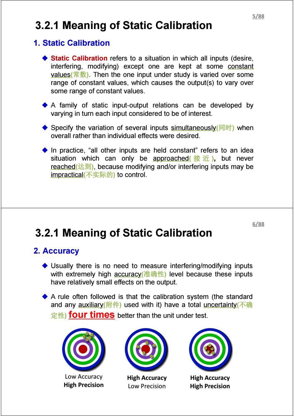
5/88 3.2.1 Meaning of Static Calibration 1.Static Calibration Static Calibration refers to a situation in which all inputs (desire, interfering,modifying)except one are kept at some constant values().Then the one input under study is varied over some range of constant values,which causes the output(s)to vary over some range of constant values. A family of static input-output relations can be developed by varying in turn each input considered to be of interest. ◆Specify the variation of several inputs simultaneously同时)when overall rather than individual effects were desired. ◆In practice,“all other inputs are held constant'”refers to an idea situation which can only be approached(接近,but never reached达到),because modifying and/.or interfering inputs may be impractical(不实际的)to control. 6/88 3.2.1 Meaning of Static Calibration 2.Accuracy Usually there is no need to measure interfering/modifying inputs with extremely high accuracy(准确性)level because these inputs have relatively small effects on the output. A rule often followed is that the calibration system (the standard and any auxiliary(附件)used with it)have a total uncertainty(不确 定性)four times better than the unit under test.. Low Accuracy High Accuracy High Accuracy High Precision Low Precision High Precision
3.2.1 Meaning of Static Calibration 1. Static Calibration Static Calibration refers to a situation in which all inputs (desire, interfering, modifying) except one are kept at some constant values(常数). Then the one input under study is varied over some range of constant values, which causes the output(s) to vary over some range of constant values. A family of static input-output relations can be developed by varying in turn each input considered to be of interest. Specify the variation of several inputs simultaneously(同时) when overall rather than individual effects were desired. In practice, “all other inputs are held constant” refers to an idea situation which can only be approached( 接 近 ), but never reached(达到), because modifying and/or interfering inputs may be impractical(不实际的) to control. 5/88 2. Accuracy Usually there is no need to measure interfering/modifying inputs with extremely high accuracy(准确性) level because these inputs have relatively small effects on the output. A rule often followed is that the calibration system (the standard and any auxiliary(附件) used with it) have a total uncertainty(不确 定性) four times better than the unit under test. 3.2.1 Meaning of Static Calibration Low Accuracy High Precision High Accuracy Low Precision High Accuracy High Precision 6/88
7/88 3.2.1 Meaning of Static Calibration 3.Standard A standard for a certain physical variable is often "just another" measuring device for that variable but with higher accuracy than the instrument to be calibrated. Primary Standards are considered the "state of the art",that is,the most accurate way known to measure the quantity of interest. Primary standards are developed,maintained,and improved by national laboratories as well as some large,high-tech,companies. They may also provide calibration services. ◆Lower Level standards(secondary,.tertiary(第三的),eto)are available for calibration services at national laboratories, commercial calibration laboratories,and in-house calibration laboratories associated with industrial companies,university laboratories,etc. 8/88 3.2.1 Meaning of Static Calibration 4.Calibration Procedure ①Examine the construction(构造)of the instrument,and identify and list all the possible inputs. ②Decide,as best you can,which of the inputs will be significant(显著 的;重要的)in the application for which the instrument is to be calibrated. 3Procure[Obtain (something),esp.with care or effort]apparatus (仪器;器械;装置)that will allow you to vary all the significant inputs over the ranges considered necessary.Procure standards to measure each input. 4By holding some inputs constant,varying others,and recording the output(s),develop the static input-output relations
3. Standard A standard for a certain physical variable is often “just another” measuring device for that variable but with higher accuracy than the instrument to be calibrated. Primary Standards are considered the “state of the art”, that is, the most accurate way known to measure the quantity of interest. Primary standards are developed, maintained, and improved by national laboratories as well as some large, high-tech, companies. They may also provide calibration services. Lower Level standards (secondary, tertiary( 第三的 ), etc) are available for calibration services at national laboratories, commercial calibration laboratories, and in-house calibration laboratories associated with industrial companies, university laboratories, etc. 3.2.1 Meaning of Static Calibration 7/88 4. Calibration Procedure ① Examine the construction(构造) of the instrument, and identify and list all the possible inputs. ② Decide, as best you can, which of the inputs will be significant(显著 的;重要的) in the application for which the instrument is to be calibrated. ③ Procure[Obtain (something), esp. with care or effort] apparatus (仪器;器械;装置) that will allow you to vary all the significant inputs over the ranges considered necessary. Procure standards to measure each input. ④ By holding some inputs constant, varying others, and recording the output(s), develop the static input-output relations. 3.2.1 Meaning of Static Calibration 8/88
9/88 3.2.2 Measured Value versus True Value 1.How close the measured value may be to its true value? The so-called true value is,in general,unknown or unknowable. The term "true value"really refers to a value called the reference value that would be obtained if the quantity under consideration were measured by an exemplar(典型;范例)method,.that is,.a method agreed by experts as being sufficiently accurate for the purpose to which the data ultimately() will be put. ◆The measurement process consists of actually carrying out(执行),as well as possible,the instructions for performing the measurement,which are the measurement method. The data generated from a large number of repeated measurement under assumed identical conditions may be used to describe the measurement process so that,if it is used in the future,we may be able to attach some numerical estimates of error to its outputs. 10/88 3.2.2 Measured Value versus True Value 2.Statistical Control To give a meaningful description of the measurement process,the output data must form what is called a random sequence(随机序列), or in another way of saying this,the process must be in the state of statistical control. Statistical Control Statistical Process Control (SPC),is the application of statistical methods to the monitoring and control of a process to ensure that it operates at its full potential to produce conforming product.Under SPC,a process behaves predictably to produce as much conforming product as possible with the least possible waste. To speak the accuracy of an instrument,the instrument must be considered with its environment and method of use,that is,the instrument plus its inputs
3.2.2 Measured Value versus True Value 1. How close the measured value may be to its true value? The so-called true value is, in general, unknown or unknowable. The term “true value” really refers to a value called the reference value that would be obtained if the quantity under consideration were measured by an exemplar(典型;范例) method, that is, a method agreed by experts as being sufficiently accurate for the purpose to which the data ultimately(最终) will be put. The measurement process consists of actually carrying out(执行), as well as possible, the instructions for performing the measurement, which are the measurement method. The data generated from a large number of repeated measurement under assumed identical conditions may be used to describe the measurement process so that, if it is used in the future, we may be able to attach some numerical estimates of error to its outputs. 9/88 3.2.2 Measured Value versus True Value 2. Statistical Control To give a meaningful description of the measurement process, the output data must form what is called a random sequence(随机序列), or in another way of saying this, the process must be in the state of statistical control. Statistical Control = Statistical Process Control (SPC), is the application of statistical methods to the monitoring and control of a process to ensure that it operates at its full potential to produce conforming product. Under SPC, a process behaves predictably to produce as much conforming product as possible with the least possible waste. To speak the accuracy of an instrument, the instrument must be considered with its environment and method of use, that is, the instrument plus its inputs. 10/88
11/88 3.2.2 Measured Value versus True Value 3.Realization of Statistical Control In defining a calibration procedure for a specific instrument,we specify that certain inputs must be held "constant"within certain limits. These inputs,it is hoped,are the ones that contribute the largest components to the overall error of the instrument. The remaining infinite number of inputs is left uncontrolled and it is hoped that each of these individually contributes only a very small effect and that in the aggregate(form or group into a class or cluster总共; 作为总体)their effect on the instrument output will be of a random nature. If the measurement process has all the above features,the process is said to be in statistical control. 12/88 3.2.2 Measured Value versus True Value 4.Effect of Uncontrolled Input on Calibration indino 0 indino 6 Morning Afternoon 111 11 12345678910 12345678910 Trial number Trial number (a)Instrument calibration under (b)Instrument calibration under room temperature controlled room temperature Figure 3.1 Effect of Uncontrolled Input on Calibration Conclusion:If the measurement process is in reasonably good statistical control and if we repeat a given measurement (or calibration point)over and over,we will generate a set of data exhibiting random scatter
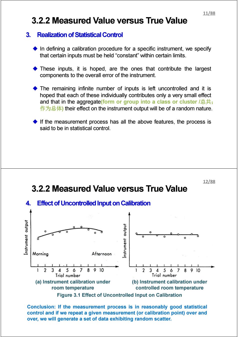
3.2.2 Measured Value versus True Value 3. Realization of Statistical Control In defining a calibration procedure for a specific instrument, we specify that certain inputs must be held “constant” within certain limits. These inputs, it is hoped, are the ones that contribute the largest components to the overall error of the instrument. The remaining infinite number of inputs is left uncontrolled and it is hoped that each of these individually contributes only a very small effect and that in the aggregate(form or group into a class or cluster /总共; 作为总体) their effect on the instrument output will be of a random nature. If the measurement process has all the above features, the process is said to be in statistical control. 11/88 3.2.2 Measured Value versus True Value 4. Effect of Uncontrolled Input on Calibration (a) Instrument calibration under room temperature (b) Instrument calibration under controlled room temperature Figure 3.1 Effect of Uncontrolled Input on Calibration Conclusion: If the measurement process is in reasonably good statistical control and if we repeat a given measurement (or calibration point) over and over, we will generate a set of data exhibiting random scatter. 12/88

13/88 3.2.2 Measured Value versus True Value 5.Calibration and Application Conditions Desired Input: 习Pressure Other possible Inputs: Temperature,acceleration,vibration,etc. It is important to carefully consider the relationship between the calibration conditions and the actual application conditions. Pointer Fluid Piston Piston rod Spring Linkage and scale Primary Vorioble- Motion Variable- Motion Dato- Pressure Force sensing conversion tronsmission conversion Measured element element element element element element Figure 3.2 Pressure Gauge 14/88 3.2.3 Some Basic Statistics(统计学) 1.Probability Cumulative Probability Trial Number Scale Reading(kPa) 1 10.20 True Pressure (Reference Value)=10+.001kPa 2 10.20 Ambient Temperature=20±1℃ 3 10.26 Acceleration=0 Vibration=0 4 10.20 5 10.22 6 10.13 7 9.97 8 10.12 9 10.09 9.809.85g909.9510001005101010.5102010.25103010350.4010.4510.50 scale reading.kPa 10 9.90 Distribution of Data 11 10.05 f(x)=Z 12 10.17 13 10.42 14 10.21 F(x) Probability Distribution 15 10.23 1.0 16 10.11 17 9.98 18 10.10 Cumulative Probability Distribution 19 10.04 Pressure-Gage Calibration Data 20 9.81
3.2.2 Measured Value versus True Value 5. Calibration and Application Conditions Desired Input: Pressure Other possible Inputs: Temperature, acceleration, vibration, etc. Figure 3.2 Pressure Gauge It is important to carefully consider the relationship between the calibration conditions and the actual application conditions. 13/88 Cumulative Probability Distribution Distribution of Data 3.2.3 Some Basic Statistics(统计学) 1. Probability & Cumulative Probability Trial Number Scale Reading(kPa) 1 10.20 2 10.20 3 10.26 4 10.20 5 10.22 6 10.13 7 9.97 8 10.12 9 10.09 10 9.90 11 10.05 12 10.17 13 10.42 14 10.21 15 10.23 16 10.11 17 9.98 18 10.10 19 10.04 20 9.81 TruePressure(Reference Value) = 10±.001kPa Ambient Temperature = 20±1℃ Acceleration = 0 Vibration = 0 Pressure - Gage Calibration Data Probability Distribution 14/88
15/88 3.2.3 Some Basic Statistics(统计学) 1.Probability Cumulative Probability (Continued) mumber of readings in an interval)/(total number of readings) .(3.1) Width of interval When the width of interval-→O,we have the probability density function概率密度函数: Z=f(x) And the probabilityofreadinglying betweena&p(a=f(x)dx(3.2) Cumulative distribution function(累积分布函数):F(x)兰∫nf(x)dce ..(3.3) The most useful density function or distribution is the normal or Gaussian function: f0)=点aew-0/的 -0<X<+00 .(3.4) where u is the mean value and o is the standard deviation. 16/88 3.2.3 Some Basic Statistics(统计学) 2.Guassian Distribution ( Small value of o indicates a high Small probability that a“reading”wlbe found close to u. Gaussian distribution can never Large occur in the real world. In much practical work,Gaussian distribution is just assumed until Smallo troubles arise which justify a closer 1.0 study of the particular situation. 0.5 Figure 3.6 Gaussian Distribution o-defines the shape of the curve u-defines the position of the curve Figure 3.7 Non-Gaussian Distribution
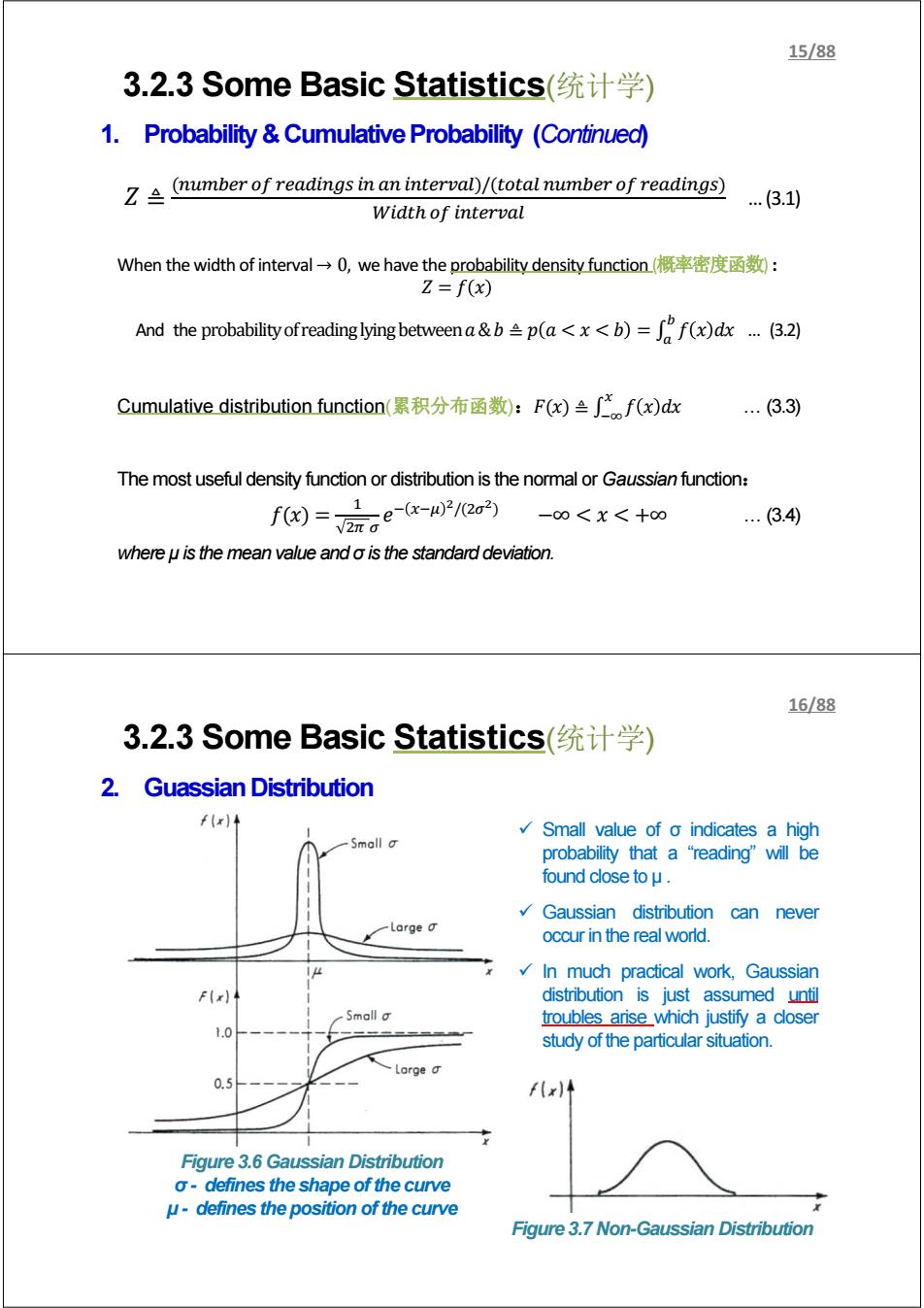
ܼ ≜ (௨ ௗ௦ ௧௩)/(௧௧ ௨ ௗ௦) ௐௗ௧ ௧௩ … (3.1) When the width of interval → 0, we have the probability density function (概率密度函数) : ݔ ݂=ܼ ௫ ݔ݀ ݔ ݂ ≜ (ݔ)ܨ:(累积分布函数(function distribution Cumulative ିஶ … (3.3) The most useful density function or distribution is the normal or Gaussian function: ଵ) = ݔ)݂ ଶగ ఙ ݁ି ௫ିఓ మ/(ଶఙమ) −∞ 3.4) where μ is the mean value and σ is the standard deviation. And the probability of reading lying between ܽ & ܾ ≜ >ܽ ݔ = ܾ> ݂ ݔ݀ ݔ … (3.2) 3.2.3 Some Basic Statistics(统计学) 1. Probability & Cumulative Probability (Continued) 15/88 Figure 3.6 Gaussian Distribution σ - defines the shape of the curve μ - defines the position of the curve Figure 3.7 Non-Gaussian Distribution 9 Small value of σ indicates a high probability that a “reading” will be found close to μ . 9 Gaussian distribution can never occur in the real world. 9 In much practical work, Gaussian distribution is just assumed until troubles arise which justify a closer study of the particular situation. 3.2.3 Some Basic Statistics(统计学) 2. GuassianDistribution 16/88
17/88 3.2.3 Some Basic Statistics(统计学) 3.Testing for an Approximate Gaussian Distribution FIx)↑ Uniformly graduated scale 1.00 Probability graph paper:a specially scaled 0.75 graph paper which is so constructed that the graph of the normal distribution function is 0.50 represented on it by a straight line. 0.25 0 Distort the vertical scale of the accumulative distribution function graph to make the curve as a straight line; F(x) Uniformly graduated scale Distorted √The ordinate(纵坐标)of any point scale represents the probability that a reading will be less than the abscissa横坐标of 0.50 that particular point. Figure 3.8 Rectification(矫正;改正)of Gaussian Curve 18/88 3.2.3 Some Basic Statistics(统计学) 3.Testing for an Approximate Gaussian Distribution(continued) Point(☒+S,84.1% Sample mean value京兰2&i N (3.5) Where X;individual reading ..(3.6) .0 Point(区,50%N N Total number ofreadings ...(3.7) Sample Standard Deviation: 30 S (Xi-X)2 20 ..(3.8) N-1 014 0.01 Figure 3.9a 96 97 98 9.9 10.0 10.1 10.2 10.3 10.4 Graphical Check of Gaussian Distribution Value of an individual reading.kPa (ol (Calibration Data Shown in Figure 3.3a)
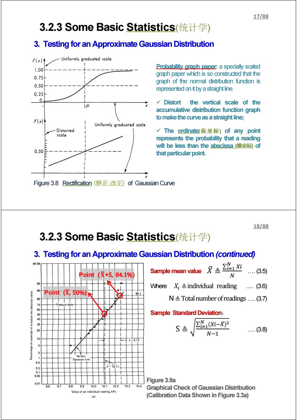
3.2.3 Some Basic Statistics(统计学) 3. Testing for an Approximate Gaussian Distribution Figure 3.8 Rectification (矫正;改正) of Gaussian Curve Probability graph paper: a specially scaled graph paper which is so constructed that the graph of the normal distribution function is representedonitbyastraightline. 9 Distort the vertical scale of the accumulative distribution function graph tomakethecurveasastraightline; 9 The ordinate(纵坐标) of any point represents the probability that a reading will be less than the abscissa (横坐标) of thatparticularpoint. 17/88 Figure 3.9a Graphical Check of Gaussian Distribution (Calibration Data Shown in Figure 3.3a) Sample mean value ܺ̅≜ ∑ ಿ సభ ே …. (3.5) Where ܺ ≜ individual reading …. (3.6) N ≜ Total number of readings …. (3.7) Sample Standard Deviation: S ≜ ∑ (ି̅ ) ಿ మ సభ ேିଵ …. (3.8) Point (܆ഥ, 50%) Point (܆ഥ+S, 84.1%) 3.2.3 Some Basic Statistics(统计学) 3. Testing for an Approximate Gaussian Distribution (continued) 18/88
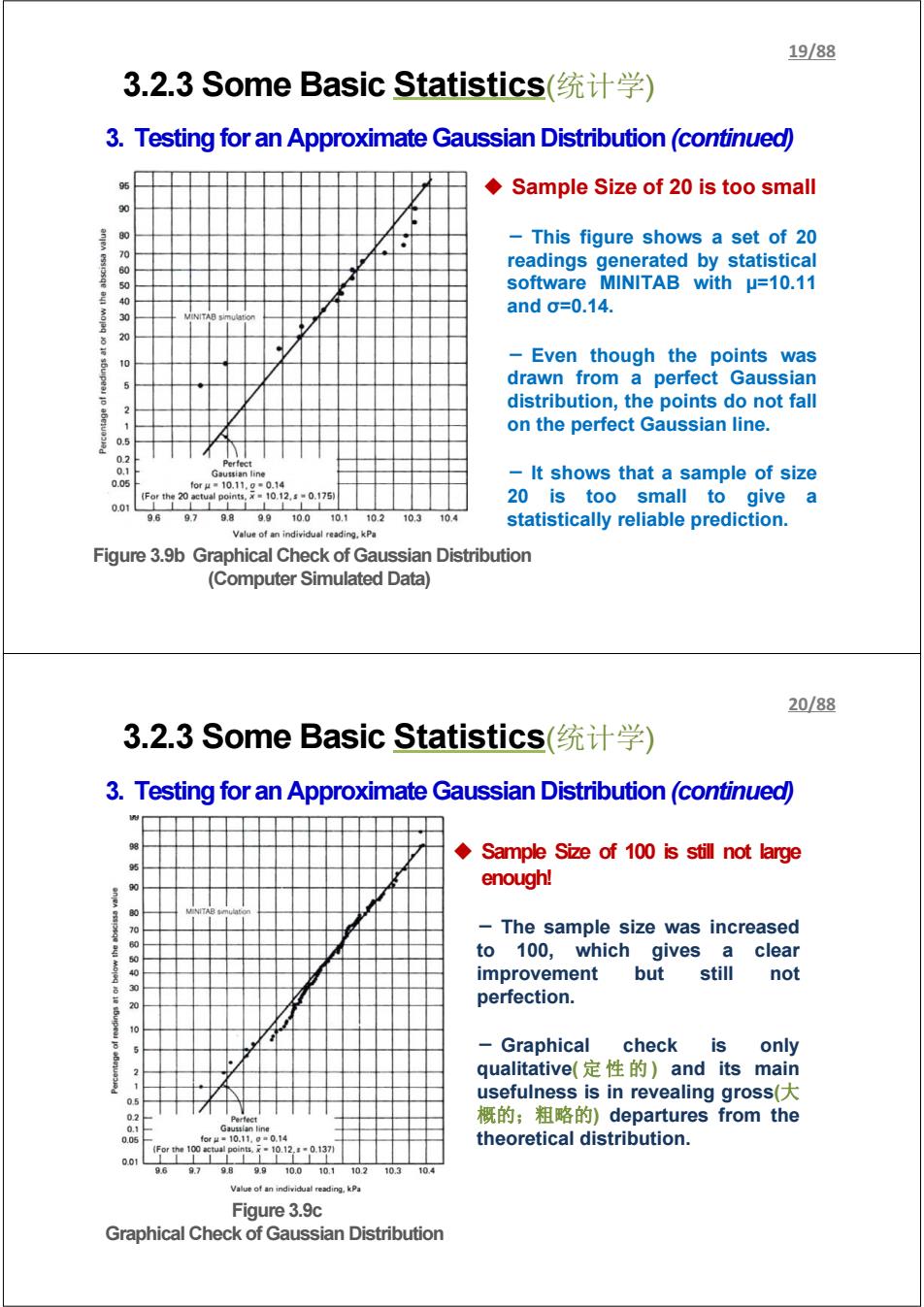
19/88 3.2.3 Some Basic Statistics(统计学) 3.Testing for an Approximate Gaussian Distribution (continued) Sample Size of 20 is too small 90 This figure shows a set of 20 70 60 readings generated by statistical 50 software MINITAB with u=10.11 and0=0.14. 3 VINITAB simu -Even though the points was drawn from a perfect Gaussian 5 distribution,the points do not fall on the perfect Gaussian line. 05 0.2 Perfect 0.1 Gaussian line 0.05 It shows that a sample of size for4=10.11.9=0.14 20 is too small to give a 0.01L 969.79.89.910.010.110.210.3 10.4 statistically reliable prediction. Value of an individual reading.kPa Figure 3.9b Graphical Check of Gaussian Distribution (Computer Simulated Data) 20/88 3.2.3 Some Basic Statistics(统计学) 3.Testing for an Approximate Gaussian Distribution(continued) Sample Size of 100 is still not large enough! 3 70 The sample size was increased to 100,which gives a clear 4 improvement but still not 20 perfection. 100 Graphical check is only qualitative(定性的)and its main usefulness is in revealing gross( 3 概的;粗略的)departures from the 01 Gaussian line 0.0 foeh-10.11.9m0.14 theoretical distribution. 001 96 9.7989910.0101102103 Value of an individual reading.kPa Figure 3.9c Graphical Check of Gaussian Distribution
Figure 3.9b Graphical Check of Gaussian Distribution (Computer Simulated Data) Sample Size of 20 is too small - This figure shows a set of 20 readings generated by statistical software MINITAB with μ=10.11 and σ=0.14. - Even though the points was drawn from a perfect Gaussian distribution, the points do not fall on the perfect Gaussian line. - It shows that a sample of size 20 is too small to give a statistically reliable prediction. 3.2.3 Some Basic Statistics(统计学) 3. Testing for an Approximate Gaussian Distribution (continued) 19/88 Figure 3.9c Graphical Check of Gaussian Distribution Sample Size of 100 is still not large enough! - The sample size was increased to 100, which gives a clear improvement but still not perfection. - Graphical check is only qualitative( 定性的 ) and its main usefulness is in revealing gross(大 概的;粗略的) departures from the theoretical distribution. 3.2.3 Some Basic Statistics(统计学) 3. Testing for an Approximate Gaussian Distribution (continued) 20/88