Chapter 4 Numerical Methods in Kinematics Determination of an assembled configuration of a system Giving estimates for the position and orientation of each component Giving the independent constraint equations The use of rapidly convergent and efficient numerical methods to solve the kinematic position equations Solution of the velocity equations Solution of the acceleration equations
• Determination of an assembled configuration of a system § Giving estimates for the position and orientation of each component § Giving the independent constraint equations • The use of rapidly convergent and efficient numerical methods to solve the kinematic position equations • Solution of the velocity equations • Solution of the acceleration equations
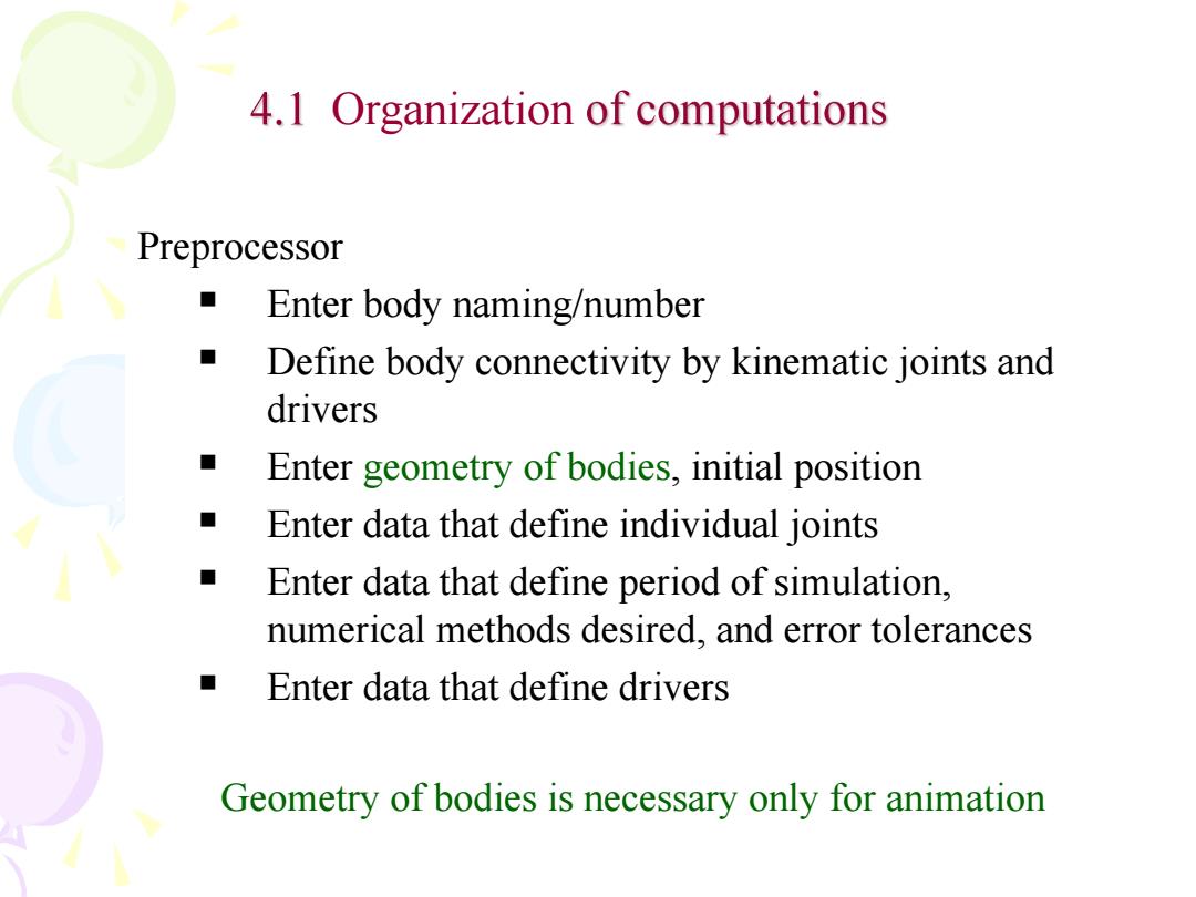
4.1 Organization of computations Preprocessor ■ Enter body naming/number Define body connectivity by kinematic joints and drivers Enter geometry of bodies,initial position Enter data that define individual joints Enter data that define period of simulation, numerical methods desired,and error tolerances Enter data that define drivers Geometry of bodies is necessary only for animation
Organization Preprocessor § Enter body naming/number § Define body connectivity by kinematic joints and drivers § Enter geometry of bodies, initial position § Enter data that define individual joints § Enter data that define period of simulation, numerical methods desired, and error tolerances § Enter data that define drivers Geometry of bodies is necessary only for animation

4.1 Organization of computations Kinematic analysis program Construct equations and matrices for kinematic analysis Assemble mechanism or declare infeasible design Identify and eliminate redundant constraint Carry out position,velocity,and acceleration analysis Postprocessor ■ Print alphanumeric results Plot curves Transmit graphic animation to terminal screen
Kinematic analysis program § Construct equations and matrices for kinematic analysis § Assemble mechanism or declare infeasible design § Identify and eliminate redundant constraint § Carry out position, velocity, and acceleration analysis Postprocessor § Print alphanumeric results § Plot curves § Transmit graphic animation to terminal screen 4.1 Organization of computations
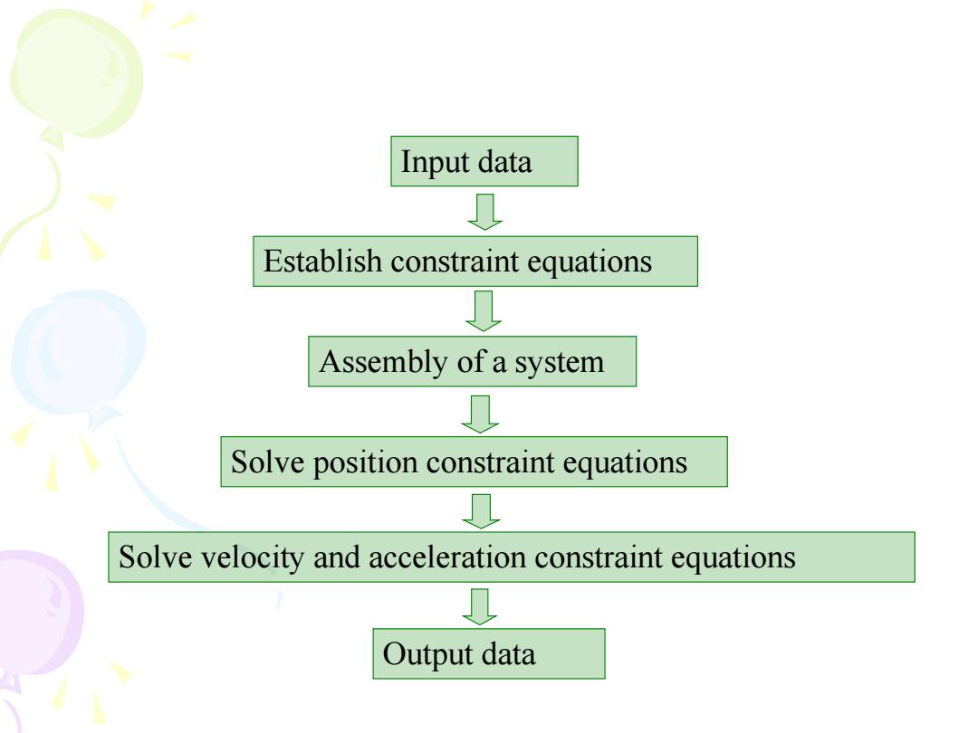
Input data 0 Establish constraint equations 0 Assembly of a system L Solve position constraint equations 见 Solve velocity and acceleration constraint equations Output data
Input data Establish constraint equations Assembly of a system Solve velocity and acceleration constraint equations Output data Solve position constraint equations

4.2 Evaluation of constraint equations and Jacobian Input data Establish constraint equations
4.2 Evaluation of constraint equations and Jacobian Input data Establish constraint equations

Input data Input the body and joint number Input initial position of each body Input joint kind and driving information Q Input inner and outer body number for each joint Input relative position vectors of the joint points Input kinematic coefficients Q Input driving coefficients (only for driving constraints
Input data Input the body and joint number Input initial position of each body Input joint kind and driving information Input inner and outer body number for each joint Input relative position vectors of the joint points Input kinematic coefficients Input driving coefficients (only for driving constraints

Establish constraint equations Derive position constraint equations 见 Calculate Jacobian matrix 夏 Calculate velocity right terms 0 Calculate acceleration right terms
Establish constraint equations Derive position constraint equations Calculate Jacobian matrix Calculate velocity right terms Calculate acceleration right terms
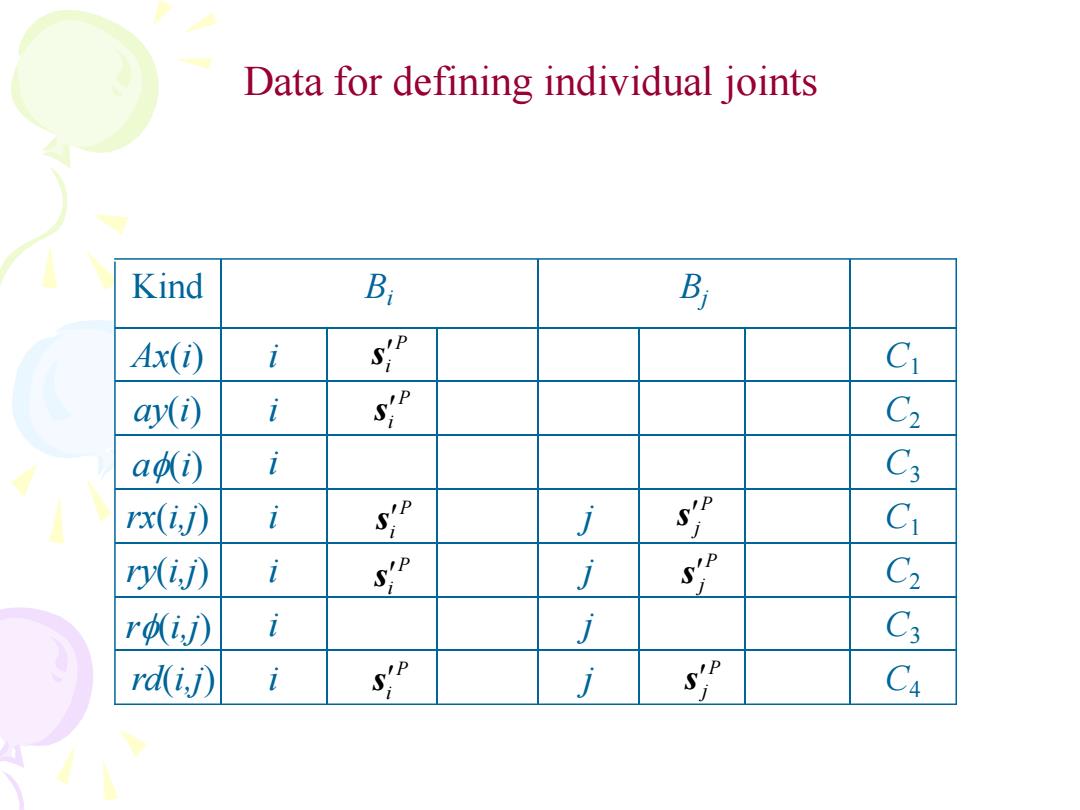
Data for defining individual joints Kind B B Ax(i) i Ci ay(i) i s C2 adi) i C3 rx(ij) i s j Ci ry(i,i) i siP j s C2 r,) C3 rd(i,j) i s j s Ca
Data for defining individual joints i i i i i i i K Bi Bj ind C2 ry(i,j) j C1 rx(i,j) j C4 rd(i,j) j C3 rf(i,j) j af(i) C3 ay C2 (i) Ax C1 (i) P i s P j s P i s P i s P i s P i s P j s P j s
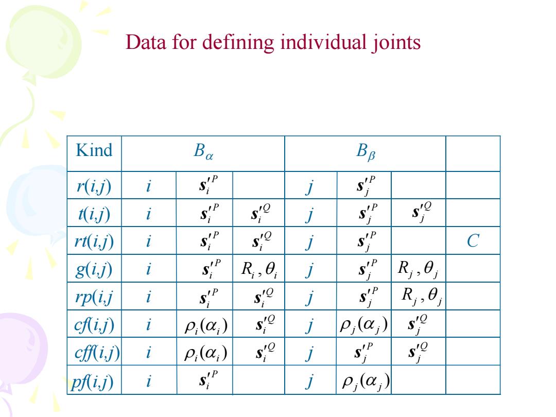
Data for defining individual joints Kind Ba Bp r() i SiP s tij i siP so j s s rt(ij) i P so j C g(ij) i sip R,0 s R,0 rp(ij i s so j R,0 cfij) i p,(c) s0 j p;(a) 59 cffij) i P,(c) S0 j so p叭i) i j p,(a)
Data for defining individual joints i i i i i i i K Ba Bb ind rp(i,j j ) g(i,j) j cf (i,j) j cf(i,j) j rt(i,j) j C t(i,j) j r(i,j) j P i s P j s P j s Ri i , Rj j , Rj j , pf(i,j) Q i s Q j s i j P i s P i s P i s P i s ( ) i ai P j s Q i s Q i s Q i s Q i s P j s P j s P j s ( ) j a j Q j ( ) s i ai P i s ( ) j a j Q j s

4.3 Assembly of a system The objective is to minimize w(q,,r)=q-g)g-g)+rΦ(g,)Φ(g,to) to obtain an assembled configuration 1=q The parameter r>0 is a constant that places relative emphasis on deviation from the initial estimate q"=limg(r) Optimization calculation
The objective is to minimize 4.3 Assembly of a system ( , , ) ( , ) ( , ) 0 0 0 0 0 t r r t t T T q q q q q q q to obtain an assembled configuration a q q The parameter r 0 is a constant that places relative emphasis on deviation from the initial estimate lim (r) r a q q Optimization calculation