ME369 Modeling,Analysis and System Control-A --Lecture 141103 Week 8# Routh Criterion Ch5.7 Nov.3(M) HW3 due Steady State Error Ch5.8 Practical lecture 1-control Nov.5(W) system modeling Quiz 2 Week 9# Nov.10(M) Frequency-Introduction,Response Ch7.1 HW4 due Now.12(W)) Frequency-Nyquist Plot Ch7.3 HW5
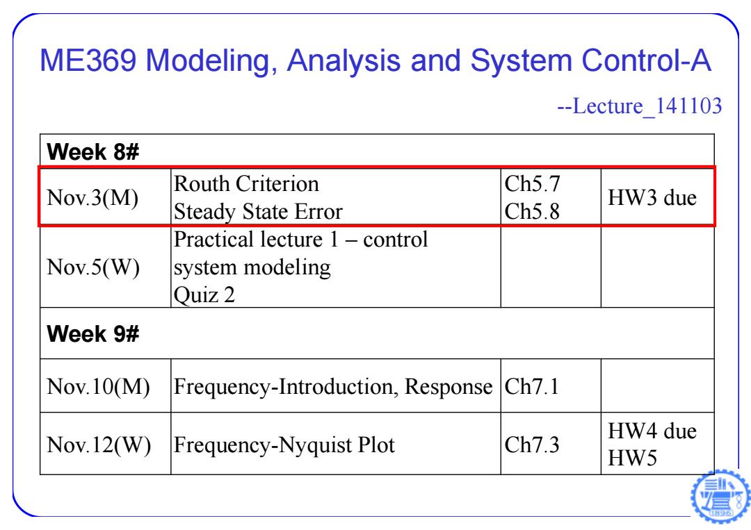
ME369 Modeling, Analysis and System Control-A --Lecture_141103 Week 8# Nov.3(M) Routh Criterion Steady State Error Ch5.7 Ch5.8 HW3 due Nov.5(W) Practical lecture 1 – control system modeling Quiz 2 Week 9# Nov.10(M) Frequency-Introduction, Response Ch7.1 Nov.12(W) Frequency-Nyquist Plot Ch7.3 HW4 due HW5
Routh Array a(s)=a,s6+a5s5+…+as+a0=0 06 ao a 43 a 0 S 4 aa4-a6凸 二A asaasa=B 0 as as as Aa3- BasC Aaaoas=D A0-0a=0 0 A A A 2 CB-AD =E Cao-40 S 二do 0 0 C ED E0-C0 S -Cao=F =0 0 0 E F Fao F0-E0 0 0 0 F F The number of sign changes of the first column elements of the Routh Array is equal to the number of unstable roots
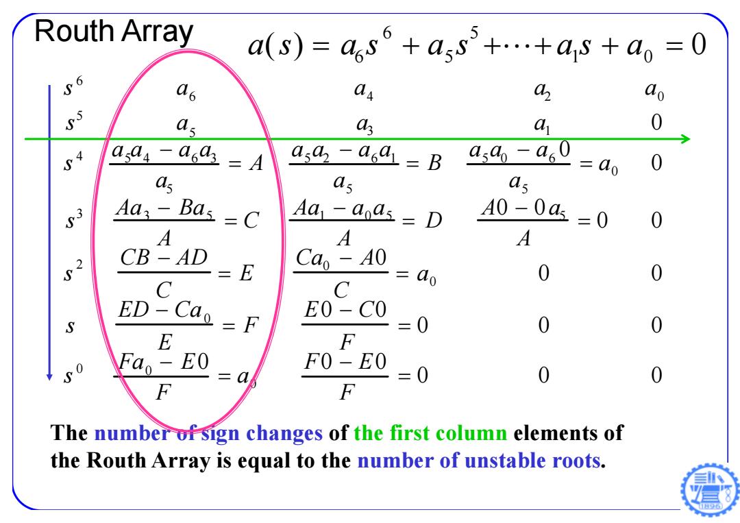
Routh Array s 6 a 6 a 4 a2 a 0 s 5 a 5 a 3 a1 0 s 4 a 5 a 4 a 6 a 3 a 5 A a 5 a2 a 6 a1 a 5 B a 5 a 0 a 6 0 a 5 a 0 0 s 3 Aa 3 Ba 5 A C Aa1 a 0 a 5 A D A 0 0 a 5 A 0 0 s 2 CB AD C E Ca 0 A 0 C a 0 0 0 s ED Ca 0 E F E 0 C 0 F 0 00 s 0 Fa 0 E 0 F a 0 F 0 E 0 F 0 00 The number of sign changes of the first column elements of the Routh Array is equal to the number of unstable roots. a ( s ) a 6 s 6 a 5 s 5 a 1 s a 0 0
Example--Verification (s-1)2(s+2)(s+3)=s4+3s3-3s2-7s+6 1 -3 6 3 -7 0 -2 6 3 0 S 20 0 S 6 Examine 1st column,of sign changes= 日96
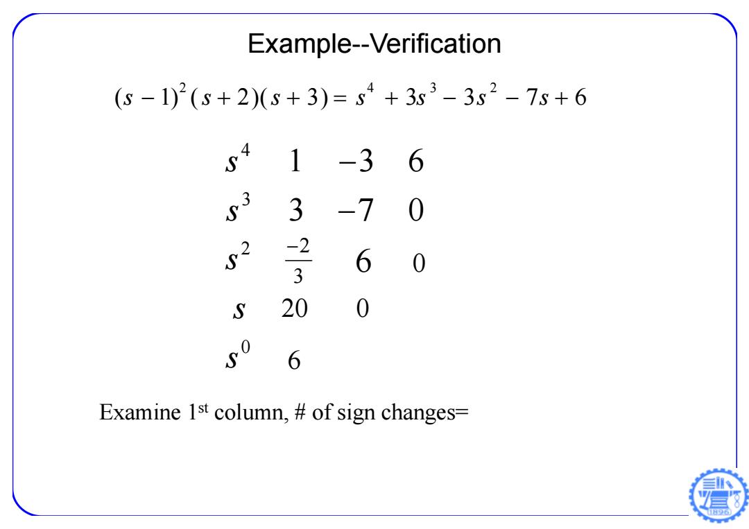
Example--Verification ( s 1) 2 ( s 2)( s 3) s 4 3 s 3 3 s 2 7 s 6 4 3 2 0 1 36 3 70 s s s s s 2 3 6 20 0 6 0 Examine 1st column, # of sign changes=

Example 10-5,Ogata,pp.541 For 3d-order polynomial: a0s3+a1s2+a2s+a3=0 The array of coefficients becomes s ao 02 a 03 a az -aoa3 0 1 s° a 0 Stable condition: Enough? a az aa;
Example 10-5, Ogata, pp.541 3 0 1 2 2 1 3 a 0 s a s a s a For 3rd-order polynomial: 0 0 3 0 1 1 1 2 0 3 1 3 2 0 2 3 s a a a a a a s s a a s a a The array of coefficients becomes Stable condition: 1 2 0 3 a a a a Enough?
Example--Verification (s2+1)(s+2)(s+3)=6s4+6s3+6s2+6s+5 665 6 6 5 S 5O Examine 1st column,of sign changes= 6
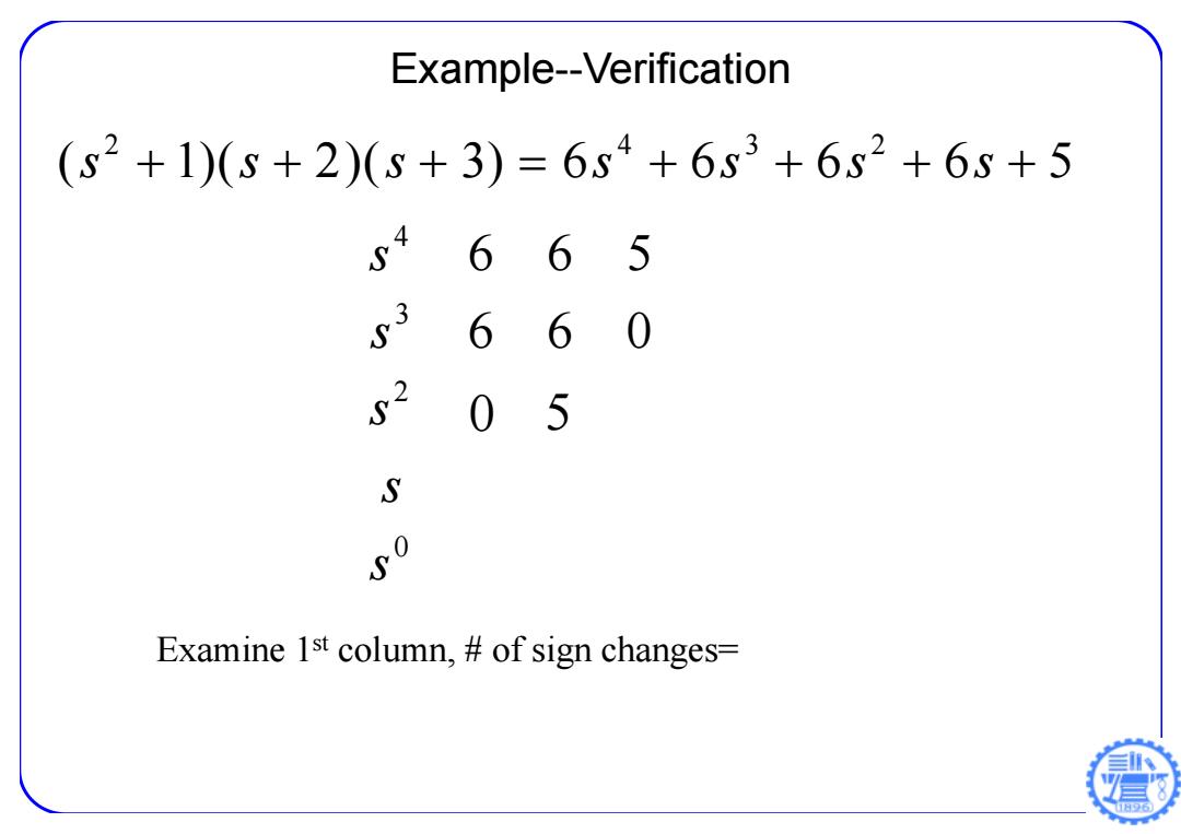
Example--Verification 2 432 ( 1)( 2)( 3) 6 6 6 6 5 s s s ssss 4 3 2 0 665 660 s s s s s 0 5 Examine 1st column, # of sign changes=
Special Case 1 When one of the terms in the first column is zero, that indicates there may be pole(s)on RHP. ·These“zero”can be replaced by a small positive number“e”and continue the process. See the two examples in Ogata,pp.542
Special Case 1 • When one of the terms in the first column is zero, that indicates there may be pole(s) on RHP. • These “zero” can be replaced by a small positive number “” and continue the process. See the two examples in Ogata, pp.542
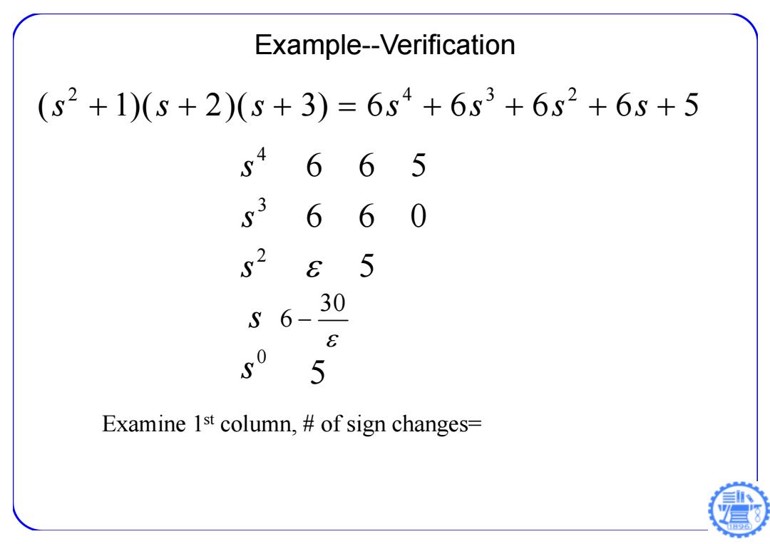
Example--Verification (s2+1)(s+2)(s+3)=6s4+6s3+6s2+6s+5 6 65 6 6 E 5 30 S E 5 5 Examine 1st column,of sign changes= 6
Example--Verification 2 432 ( 1)( 2)( 3) 6 6 6 6 5 s s s ssss 4 3 2 0 665 660 5 s s s s s 30 6 5 Examine 1st column, # of sign changes=
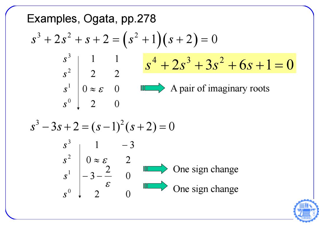
Examples,Ogata,pp.278 s3+2s2+s+2=(s2+1)(s+2)=0 s3 1 s4+2s3+3s2+6s+1=0 s2 2 2 s 0 0 A pair of imaginary roots 2 s3-3s+2=(s-1)2(s+2)=0 1 -3 s2 0≈8 2 -3 2 0 →One sign change → 2 One sign change
2 0 0 0 2 2 1 1 0 1 2 3 s s s s 32 2 s ss s s 2 2 1 20 Examples, Ogata, pp.278 2 0 0 2 3 0 2 1 3 0 1 2 3 s s s s A pair of imaginary roots One sign change One sign change 2 3 6 1 0 4 3 2 s s s s 3 2 ss s s 3 2 ( 1) ( 2) 0
Special Case 2 If all the coefficients in any row become all zero, that indicate poles in mirror image with respect to the origin. The evaluation can be continued by forming an auxiliary polynomial,by taking the coefficients of the last non-zero row. The all-zero row is then replaced by the coefficients of the derivative of the auxiliary polynomial
Special Case 2 • If all the coefficients in any row become all zero, that indicate poles in mirror image with respect to the origin. • The evaluation can be continued by forming an auxiliary polynomial, by taking the coefficients of the last non-zero row. • The all-zero row is then replaced by the coefficients of the derivative of the auxiliary polynomial
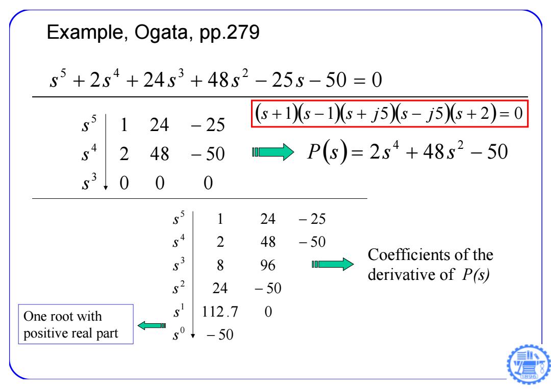
Example,Ogata,pp.279 s5+2s4+24s3+48s2-255-50=0 1 24-25 (6+10s-1s+j5s-j5g+2)=0 2 48-50 →P(s)=2s4+48s2-50 53 ,0 0 0 1 24 -25 2 48 -50 Coefficients of the 8 96 derivative of P(s) 24 -50 One root with 112.7 0 positive real part 50 -50
Example, Ogata, pp.279 2 24 48 25 50 0 5 4 3 2 s s s s s 0 0 0 2 48 50 1 24 25 3 4 5 s s s 2 48 50 4 2 P s s s 50 112.7 0 24 50 8 96 2 48 50 1 24 25 0 1 2 3 4 5 s s s s s s Coefficients of the derivative of P(s) One root with positive real part s 1 s 1 s j 5 s j 5 s 2 0