
ME369 Modeling,Analysis and System Control-A --Lecture 140922 Week 2# Laplace Transform-inverse, Ch2.4, Sep.22(M) solving equation,MATLAB 2.5(4h) Dynamic systems-mechanical Ch3.1~ HW1 due Sep.24(W) electrical system modeling 3.3 HW2 Week 3#Rest Week 4# 0ct.6M)) Rest Dynamic systems- Ch3.1~ Oct.8(W) mechanical/electrical system 3.3 modeling
ME369 Modeling, Analysis and System Control-A --Lecture_140922 Week 2# Sep.22(M) Laplace Transform – inverse, solving equation, MATLAB Ch2.4, 2.5 (4th ) Sep.24(W) Dynamic systems – mechanical / electrical system modeling Ch3.1 ~ 3.3 HW1 due HW2 Week 3# Rest Week 4# Oct.6(M) Rest Oct.8(W) Dynamic systems – mechanical/electrical system modeling Ch3.1 ~ 3.3

Definition of Laplace Transform Definition of Laplace Transform The Laplace Transform of f(t)is defined as F(s)=f(t)e-dt=[f() S=0+j0 Function ft)that satisfies 1.A time continuous function; 2.Real function; 3.t)=0,for0: 4 0f(t)eh<w→limf()e=0
• Definition of Laplace Transform • The Laplace Transform of f(t) is defined as 0 ( ) ( ) [ ( )] st F s f t e dt f t L lim ( ) 0 st t f te 0 ( ) st f t e dt Definition of Laplace Transform s j Function f(t) that satisfies 1. A time continuous function; 2. Real function; 3. f(t)=0, for t<0; 4

Laplace Transform of Typical Function Exponential Function f(t)=0 fort<0 F(S)=? f(t)=Ae-a for t≥0 [f(t)=0 for t<0 Step Function F(S)=? f(t)=A for t≥0 f(t)=0 fort<0 Ramp Function F(S)=? f(t)=At for t≥0
Laplace Transform of Typical Function Exponential Function ( ) for 0 ( ) 0 for 0 f t Ae t f t t t Step Function ( ) for 0 ( ) 0 for 0 f t A t f t t Ramp Function ( ) for 0 ( ) 0 for 0 f t At t f t t F s() ? F s() ? F s() ?

Laplace Transform of Typical Function Sinusoidal Function f(t)=0 fortto Impulse Function ()=lim for0 F(S)=? i0→0t0 6(t-to)=0fort≠to δ(t-to)=∞fort=to F(s)=? Unit Impulse Function [6(t-to)dt =1 Table A.1,by Ogata
Laplace Transform of Typical Function Impulse Function Unit Impulse Function 0 0 0 0 ( ) lim for 0 ( ) 0 for 0 and t t 0 t t t A f t f t t t ( ) 1 ( ) for t t ( ) 0 for t 0 0 0 0 0 t t dt t t t t t F s() ? F s() ? ( ) sin for 0 ( ) 0 for 0 f t A t t f t t Sinusoidal Function F s() ? Table A.1, by Ogata

Important properties of the Laplace Transform(1) 1.Multiplication of f(t)by e-at LeSe"f()e"d=F(+a) Translated Function (time delay) L[f(t-a).1(t-a)=eaF(s)
Important properties of the Laplace Transform(1) ( ) ( ) ( ) L e f t e f t e dt F s t t st 0 1.Multiplication of f(t) by e-αt Translated Function (time delay) ( ) 1( ) ( ) as L ft a t a e Fs
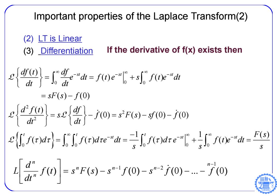
Important properties of the Laplace Transform(2) (2) LT is Linear (3) Differentiation If the derivative of f(x)exists then \离=foef+eh =sF(S)-f(0) 9到=心离0=0-0 (ddread 小蛋0o-0r7-70
Important properties of the Laplace Transform(2) (2) LT is Linear (3) Differentiation ( ) ( ) ( 0 ) ( 0 ) ... ( 0 ) 1 1 2 n n n n n n f t s F s s f s f f dt d L If the derivative of f(x) exists then 0 0 0 2 2 2 0 00 0 0 0 ( ) () () ( ) (0) ( ) (0) ( ) (0) (0) 1 1 ( ) ( ) ( ) () st st st tt t st st st df t df e dt f t e s f t e dt dt dt sF s f d f t df s f s F s sf f dt dt F f d f d e dt f d e f t e dt s s L L L L ( )s s
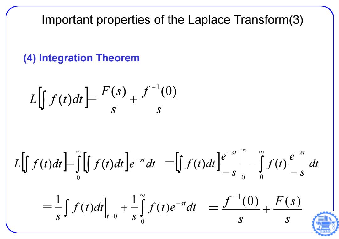
Important properties of the Laplace Transform(3) (4)Integration Theorem ff0a/'o S row-jinolo -S dt -dfe() S S
Important properties of the Laplace Transform(3) (4) Integration Theorem s f s F s L f t dt ( ) ( ) ( ) 0 1 = dt s e f t s e f t dt st st 0 0 L f t dt f t dt e dt = ( ) ( ) st 0 ( ) = ( ) 0 0 ( ) 1 ( ) 1 f t e dt s f t dt s st t = s F s s f ( 0 ) ( ) 1 =
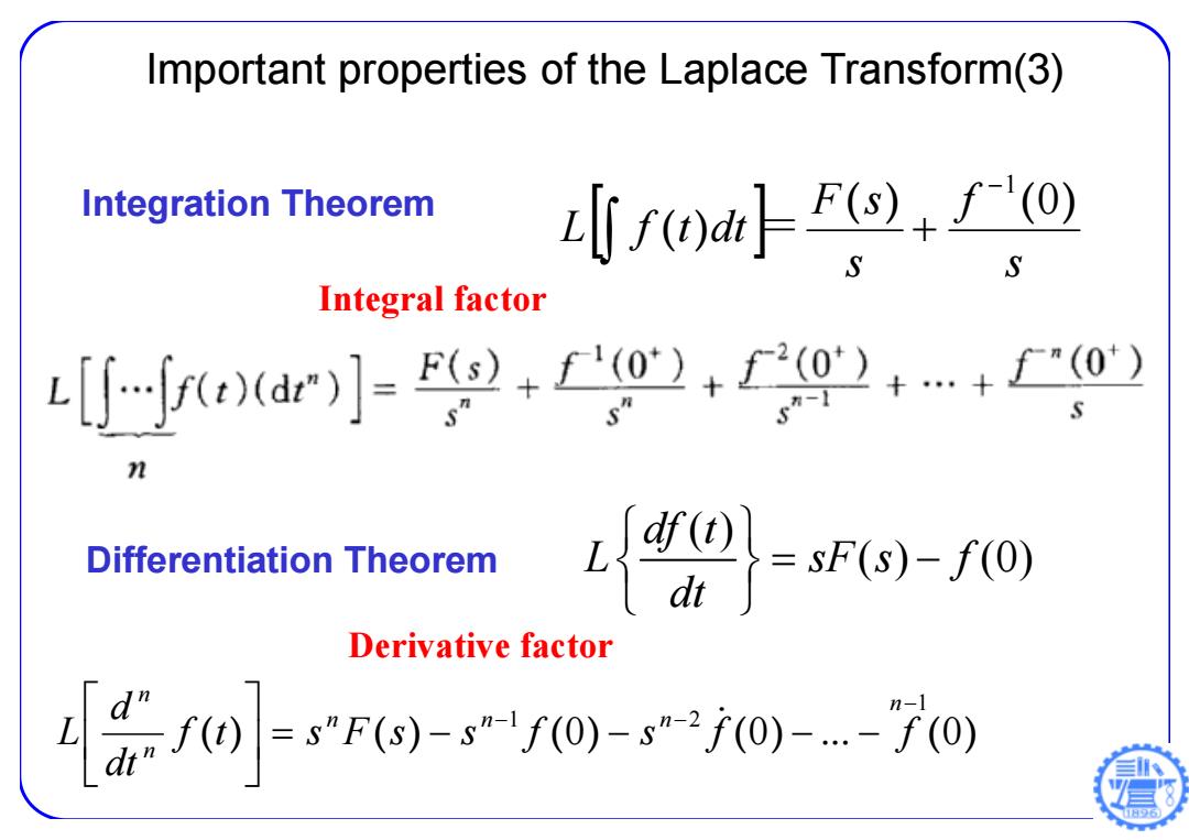
Important properties of the Laplace Transform(3) Integration Theorem rmalF+'@ Integral factor -d]小-+f八o+0+o) Differentiation Theorem t0=a-0, Derivative factor ]=7s70-f0-70
Important properties of the Laplace Transform(3) Integration Theorem s f s F s L f t dt ( ) ( ) ( ) 0 1 = ( ) ( ) (0) df t L sF s f dt Differentiation Theorem Integral factor Derivative factor ( ) ( ) ( 0 ) ( 0 ) ... ( 0 ) 1 1 2 n n n n n n f t s F s s f s f f dt d L
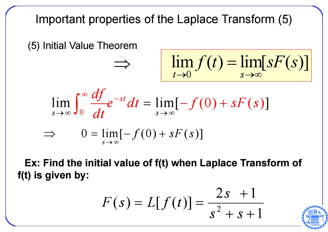
Important properties of the Laplace Transform(5) (5)Initial Value Theorem → lim f(t)=lim[sF(s)] t→0 S→00 lime-"dt=lim[-f(0)+sF(s)] dt S-> → 0=lim[-f(0)+sF(s)] S→00 Ex:Find the initial value of f(t)when Laplace Transform of f(t)is given by: 25+1 F(S)=L[f(t)]= s2+s+1
Important properties of the Laplace Transform (5) (5) Initial Value Theorem 0 lim lim[ () () 0 ] s s df st e dt f sF s dt 0 lim[ (0) ( )] s f sF s 0 lim ( ) lim[ ( )] t s f t sF s Ex: Find the initial value of f(t) when Laplace Transform of f(t) is given by: 1 2 1 ( ) [ ( )] 2 s s s F s L f t
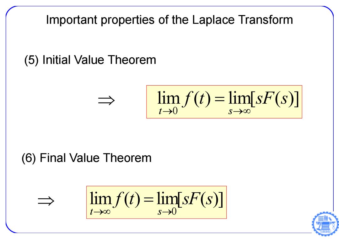
Important properties of the Laplace Transform (5)Initial Value Theorem → lim f(t)=lim[sF(s)] t->0 (6)Final Value Theorem → limf(t)=limsF(s)] s->0
Important properties of the Laplace Transform (6) Final Value Theorem 0 lim ( ) lim[ ( )] t s f t sF s (5) Initial Value Theorem 0 lim ( ) lim[ ( )] t s f t sF s