ADVANCED MACROECONOMICS Lecture 2 Solow-Swan Growth Model 电子科大经管学院马捷
ADVANCED MACROECONOMICS Lecture 2 Solow-Swan Growth Model 电子科大经管学院 马捷 1

Contents ·Introduction Mathematical Framework Graphical Representation Empirical Evidence Criticisms References 电子科大经管学院马捷 2
Contents Introduction Mathematical Framework Graphical Representation Empirical Evidence Criticisms References 电子科大经管学院 马捷 2

Introduction Developed by Robert Solow in 1956 -Extension to the Harrod-Domar model: Adding labor as a factor of production; The capital-output and capital-labor ratios are not fixed Requiring diminishing returns to labor and capital separately,and constant returns to scale for both factors combined; Introducing a time-varying technology variable distinct from capital and labor. 电子科大经管学院马捷 3
Introduction Developed by Robert Solow in 1956. Extension to the Harrod-Domar model: • Adding labor as a factor of production; • The capital-output and capital-labor ratios are not fixed • Requiring diminishing returns to labor and capital separately, and constant returns to scale for both factors combined; • Introducing a time-varying technology variable distinct from capital and labor. 电子科大经管学院 马捷 3

Five Macroeconomic Equations 0 The production function:Y:=AF(K:,L) F is stationary,continuous and twice differentiable. GDP equation Y=C+G+C+lsY Savings function:/=sY Change in capital::△KsYrδK Change in workforce:L=Lt.1(1+n)=(1+n)Lo 电子科大经管学院马捷
Five Macroeconomic Equations The production function: Yt = A t F ( Kt, L t) F is stationary, continuous and twice differentiable. GDP equation : Yt = C t + G t + I t C t + I t ≤ Yt Savings function: I t =sYt Change in capital: ∆ Kt =sYt - Kt Change in workforce: L t = L t-1(1+ n)=(1+ n ) t L 0 电子科大经管学院 马捷 4

“Neoclassical”Properties 1.F(K,L)=F(K,L),4>0. 2.Fx(K,L)>0,F(K,L)>0,F(K,L)>0, F(K,L)oc L00 Implication:F(0,L)=F(K,0)=0, F(K,L)=Fk(K,L)K+F(K,L)L or 1=8k+8L 电子科大经管学院马捷 5 元元元
“Neoclassical” Properties K L K L L L K K L L K K KK LL K L KL F K L F K L K F K L L or F F F F F K L F K L F K L F K L F K L F K L F K L ( , ) ( , ) ( , ) 1 Implication : F (0,L) F (K, 0) 0, lim lim 0. 3. lim lim , ( , ) 0, ( , ) 0. 2. ( , ) 0, ( , ) 0, ( , ) 0, 1. ( , ) ( , ), 0. 0 0 电子科大经管学院 马捷 5

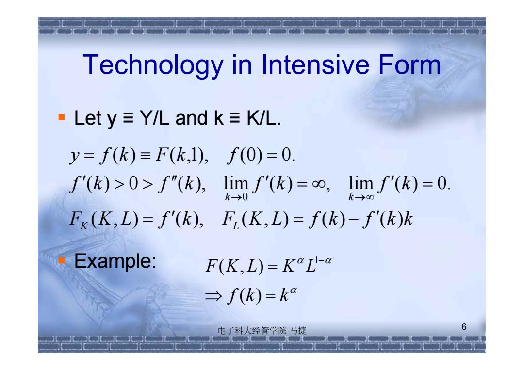
Technology in Intensive Form Lety≡Y/L and k≡KWL. y=f(k)三F(k,1),f(0)=0. '(k)>0>f"(k), im()=limf(k)=0. Fk(K,L)=f(k),F(K,L)=f(k)-f(k)k Example: F(K,L=K4L-@ →f(k)=ka 电子科大经管学院马捷 6 元元元
Technology in Intensive Form Let y ≡ Y/L and k ≡ K/L. Example: 6 F K L f k F K L f k f k k f k f k f k f k y f k F k f K L k k ( , ) ( ), ( , ) ( ) ( ) ( ) 0 ( ), lim ( ) , lim ( ) 0. ( ) ( ,1), ( 0 ) 0. 0 f k k F K L K L ( ) ( , ) 1 电子科大经管学院 马捷

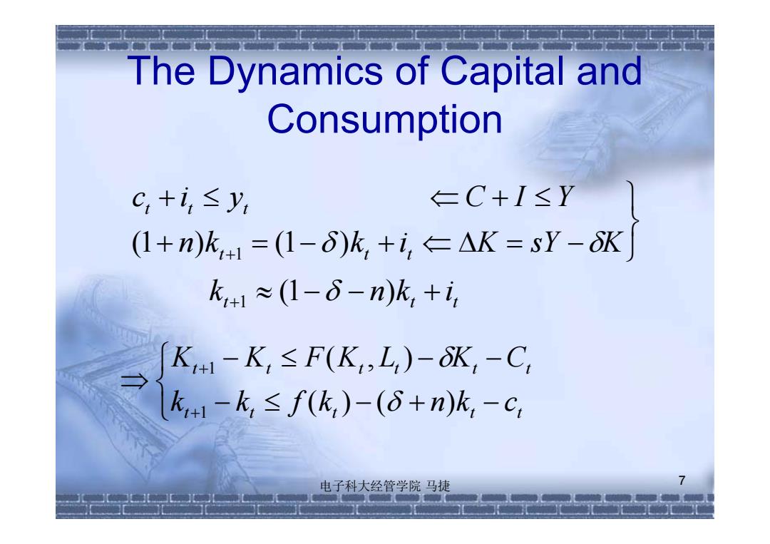
The Dynamics of Capital and Consumption C,+i,≤y, =C+I≤Y (1+n)k1=(1-δ)k,+i,←△K=sY-K k+1≈(1-δ-n)k,+i K+1-K,≤F(K,L,)-N,-C k,+1-k,≤f(k,)-(δ+n)k,-c, 电子科大经管学院马捷 元元元
The Dynamics of Capital and Consumption 7 t t t t t t t t t k n k i n k k i K sY K c i y C I Y ( 1 ) ( 1 ) ( 1 ) 1 1 t t t t t t t t t t t k k f k n k c K K F K L K C ( ) ( ) ( , ) 1 1 电子科大经管学院 马捷

Feasible and "Optimal Allocations A feasible allocation: Any c)satisfies k1≤f(k)+(1-δ-n)k,-c A "Solow-optimal"centralized allocation Any feasible allocation satisfies the resource constraint with equality and c=(1-s)f(k,) 电子科大经管学院马捷 8 元元元
Feasible and “Optimal” Allocations A feasible allocation: A “Solow-optimal” centralized allocation 8 and ( 1 ) ( ) the resource constraint with equality Any feasible allocation satisfies t t c s f k t t t t t t t k f k n k c c k ( ) ( 1 ) Any , satisfies 1 2 0 电子科大经管学院 马捷

Dynamics of the Dictatorial Economy ·The path of{k,。: k+=G(k,),G(k)≡sf(k)+(1-δ-n)k The growth rate: =k-=7k where y(k)≡s(k)-(δ+n),(k)≡f(k)/k 电子科大经管学院马捷 9
Dynamics of the Dictatorial Economy The path of : The growth rate: 9 k G k G k sf k n k t t ( ), ( ) ( ) ( 1 ) 1 t t 0 k k s k n k f k k k k k k t t t t t where ( ) ( ) ( ), ( ) ( ) / ( ), 1 电子科大经管学院 马捷

The Policy Rule ko-1 450 Gk) 01 kkk" k 电子科大经管学院马捷 10 元元
The Policy Rule 电子科大经管学院 马捷 10