Synaptic DynamicsII:Supervised Learning The Backpropagation Algorithm and Spport Vector Machines JingLIU 2004.11.3
Synaptic DynamicsII : Supervised Learning The Backpropagation Algorithm and Spport Vector Machines JingLIU 2004.11.3

History of BP Algorithm Rumelhart [1986]popularized the BP algorithm in the Paralle/Distributed Processing edited volume in the late 1980's. ■ BP algorithm overcame the limitations of the perceptron algorithm,limitations that Minsky and Papert[1969]had carefully enumerated. BP's popularity begot waves of criticism.BP algorithm often failed to converge,and at best converged to local error minima. The wave of criticism challenged BP's historical priority. The wave of criticism challenge whether the BP learning was new.The algorithm not offer a new kind of learning
History of BP Algorithm ◼ Rumelhart [1986]popularized the BP algorithm in the Parallel Distributed Processing edited volume in the late 1980’s. ◼ BP algorithm overcame the limitations of the perceptron algorithm, limitations that Minsky and Papert[1969] had carefully enumerated. ◼ BP’s popularity begot waves of criticism. BP algorithm often failed to converge, and at best converged to local error minima. ◼ The wave of criticism challenged BP’s historical priority. ◼ The wave of criticism challenge whether the BP learning was new. The algorithm not offer a new kind of learning
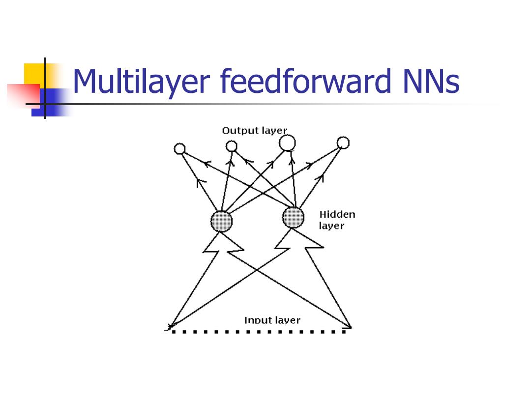
Multilayer feedforward NNs Output layer Hidden layer Input layer ■■■■■■■■■■■■■
Multilayer feedforward NNs
Feedforward Sigmoidal Representation Theorems Feedforward sigmoidal architectures can in principle represent any Borel-measurable function to any desired accuracy-if the network contains enough hidden"neurons between the input and output neuronal fields. So the MLP can solve the problems of nonlinear separable problems and function approximate
Feedforward Sigmoidal Representation Theorems ◼ Feedforward sigmoidal architectures can in principle represent any Borel-measurable function to any desired accuracy—if the network contains enough “hidden” neurons between the input and output neuronal fields. ◼ So the MLP can solve the problems of nonlinear separable problems and function approximate
Feedforward Sigmoidal Representation Theorems We can explain the theorem in the following two aspects: To improve the NNs'classification ability,we must use multilayer networks,at least one hidden layers. One the other hand,when feedforward-sigmoidal neural networks finely approximate complicated functions,the networks may suffer a like "explosion"of hidden neurons and interconnecting synapses
Feedforward Sigmoidal Representation Theorems ◼ We can explain the theorem in the following two aspects: ◼ To improve the NNs’ classification ability, we must use multilayer networks, at least one hidden layers. ◼ One the other hand, when feedforward –sigmoidal neural networks finely approximate complicated functions, the networks may suffer a like “explosion” of hidden neurons and interconnecting synapses

How can a MLP learn? We know only the random sample (xi,Y)and the vector error Y-N(X) OMSE △m,k)=-c4am, aSE(k) Am(k)=-Cx my Y-N(X
How can a MLP learn? ◼ We know only the random sample (xi ,Yi ) and the vector error Yi -N(Xi ) ij ij k m m k c = − MSE ( ) ij ij k m k m k c = − SE( ) ( ) Xi Yi-N(Xi)
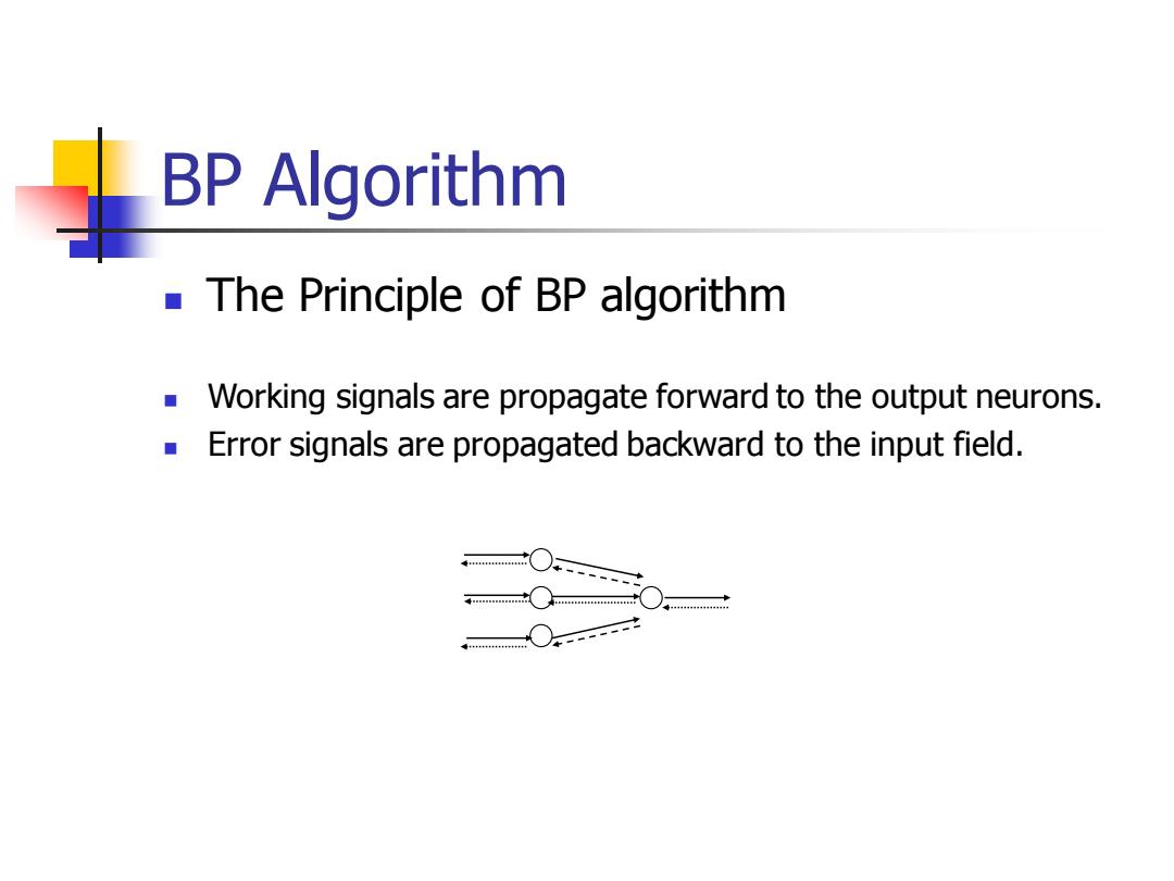
BP Algorithm The Principle of BP algorithm Working signals are propagate forward to the output neurons. Error signals are propagated backward to the input field
BP Algorithm ◼ The Principle of BP algorithm ◼ Working signals are propagate forward to the output neurons. ◼ Error signals are propagated backward to the input field
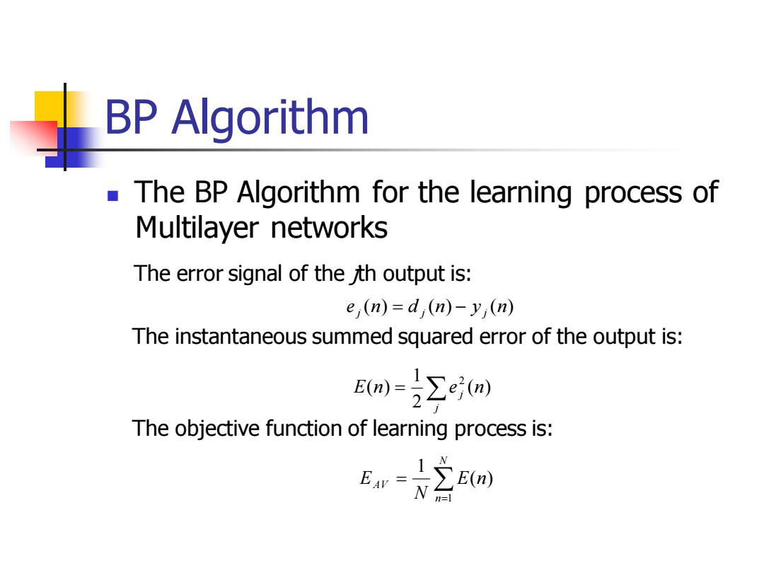
BP Algorithm The BP Algorithm for the learning process of Multilayer networks The error signal of the th output is: e,(n)=d,(n)-y,(n) The instantaneous summed squared error of the output is: m=∑em The objective function of learning process is: Hn()
BP Algorithm ◼ The BP Algorithm for the learning process of Multilayer networks The error signal of the jth output is: The instantaneous summed squared error of the output is: The objective function of learning process is: e (n) d (n) y (n) j = j − j = j E n e j (n) 2 1 ( ) 2 = = N n AV E n N E 1 ( ) 1
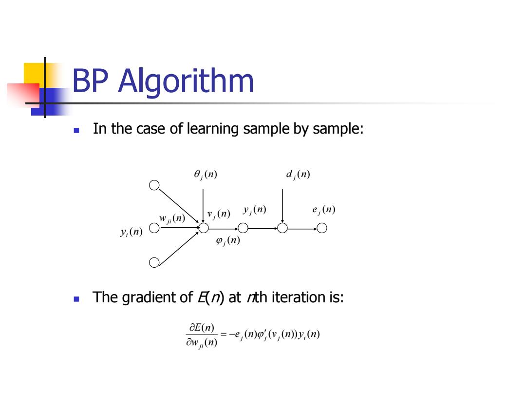
BP Algorithm In the case of learning sample by sample: 0,(n) d,(n) y,m)y,(n) e,(n) y(n)○ ○ p,(n) The gradient of at nth iteration is: E(n) 50=e,mp心m@
BP Algorithm ◼ In the case of learning sample by sample: ◼ The gradient of E(n) at nth iteration is: v (n) j y (n) i (n) j y (n) j d (n) j e (n) j w (n) ji ( ) ( ( )) ( ) ( ) ( ) e n v n y n w n E n j j j i ji = − (n) j

BP Algorithm The modification quantity of weight w is: E(n)--n,(n)y.(n) △w,m=-naNm where δ,(n)=e,(n)p(v,(n) (1) For j is an output neuron:5,(n)=(d,(n)-y (n)((m)) (2) For j is a hidden neuron: 6,0m= aEmo'v,n》 ay,(n))' d,(m)=py,(n∑d(m)wg(m) [△wu]=[n][δ,(n][y,(n)]
BP Algorithm ◼ The modification quantity of weight wji is: where (1) For j is an output neuron: (2) For j is a hidden neuron: ( ) ( ) ( ) ( ) ( ) n y n w n E n w n j i ji ji = − = − (n) e (n) (v (n)) j j j j = = k j (n) j (v j (n)) k (n)wkj (n) (n) (d (n) y (n)) (v (n)) j j j j j = − ( ( )) ( ) ( ) ( ) v n y n E n n j j j = − [ w ] [ ] [ (n)] [ y (n)] ij j i = • •