
电子种越女学 University of Electroale Science and Technelery of China 986 Chapter 8 Fast Convolution Dr.Ling National Key Lab of Science and Technology on Communications
Chapter 8 Fast Convolution Dr. Ling National Key Lab of Science and Technology on Communications
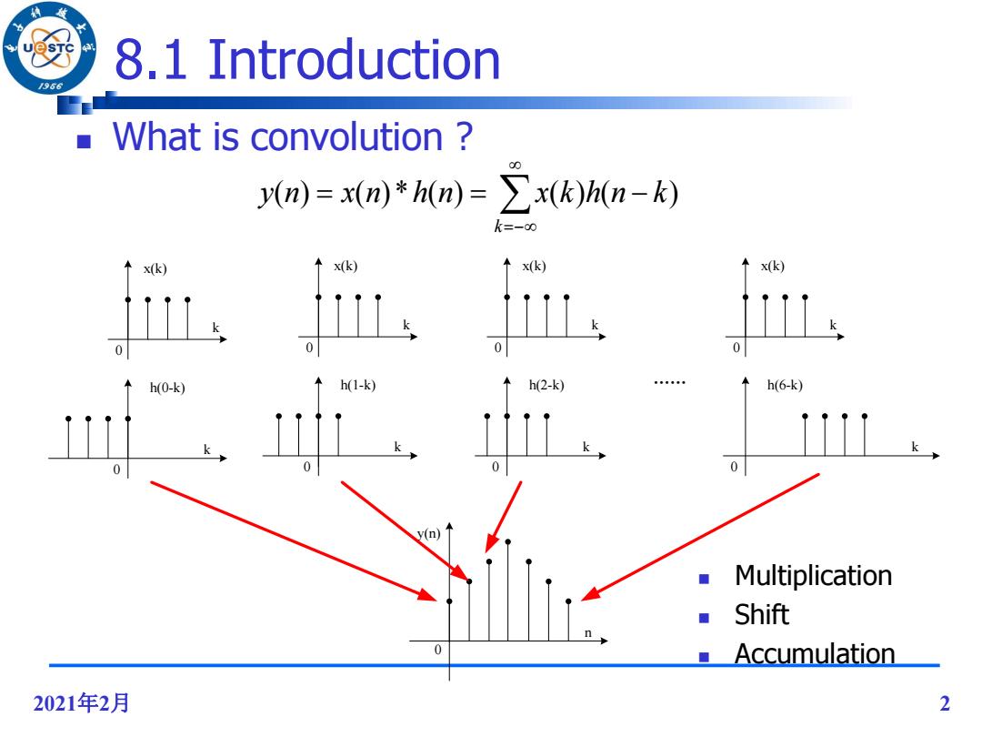
8.1 Introduction 986 What is convolution 00 y(n)=x(n)*h(n)=>x(k)h(n-k) k=-00 x(k) ↑x(k) ↑x(k) x(k) h(0-k) h(1-k) h(2-k) h(6-k) 0 y(n) Multiplication Shift n ■Accumulation 2021年2月 2
2021年2月 2 k k 0 0 x(k) h(0-k) k k 0 0 x(k) h(1-k) k k 0 0 x(k) h(2-k) k k 0 0 x(k) h(6-k) n y(n) 0 …… 8.1 Introduction Multiplication Shift Accumulation What is convolution ? k y(n) x(n)*h(n) x(k)h(n k)

Fast convolution /96 Fast Convolution:implementation of convolution algorithm using fewer multiplication operations by algorithmic strength reduction. Algorithmic Strength Reduction:Number of strong operations(such as multiplication operations)is reduced at the expense of an increase in the number of weak operations (such as addition operations).These are best suited for implementation using either programmable or dedicated hardware. 2021年2月 3
2021年2月 3 Fast convolution Fast Convolution: implementation of convolution algorithm using fewer multiplication operations by algorithmic strength reduction. Algorithmic Strength Reduction: Number of strong operations (such as multiplication operations) is reduced at the expense of an increase in the number of weak operations (such as addition operations). These are best suited for implementation using either programmable or dedicated hardware

966 The examples of algorithms strength reduction e+if=(a+jb)(c+jd)=(ac-bd)+j(bc+ad) Direct implementation 调 4 multiplications and 2 additions 2021年2月 4
2021年2月 4 The examples of algorithms strength reduction Direct implementation e jf (a jb)(c jd ) (ac bd) j(bc ad) 4 multiplications and 2 additions
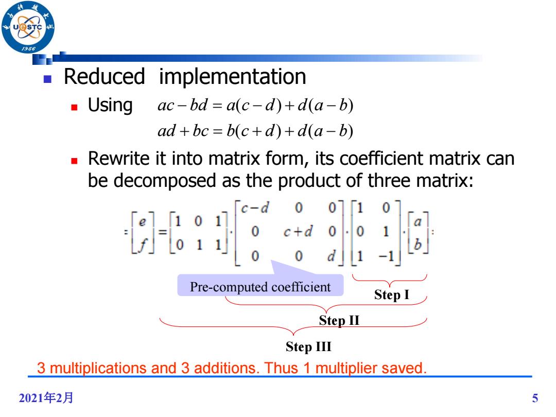
/966 Reduced implementation Using ac-bd a(c-d)+d(a-b) ad+bc=b(c+d)+d(a-b) Rewrite it into matrix form,its coefficient matrix can be decomposed as the product of three matrix: 世服胸 Pre-computed coefficient Step I Step IⅢ Step III 3 multiplications and 3 additions.Thus 1 multiplier saved. 2021年2月 5
2021年2月 5 Reduced implementation Using Rewrite it into matrix form, its coefficient matrix can be decomposed as the product of three matrix: ( ) ( ) ( ) ( ) ad bc b c d d a b ac bd a c d d a b 3 multiplications and 3 additions. Thus 1 multiplier saved. Pre-computed coefficient Step I Step II Step III
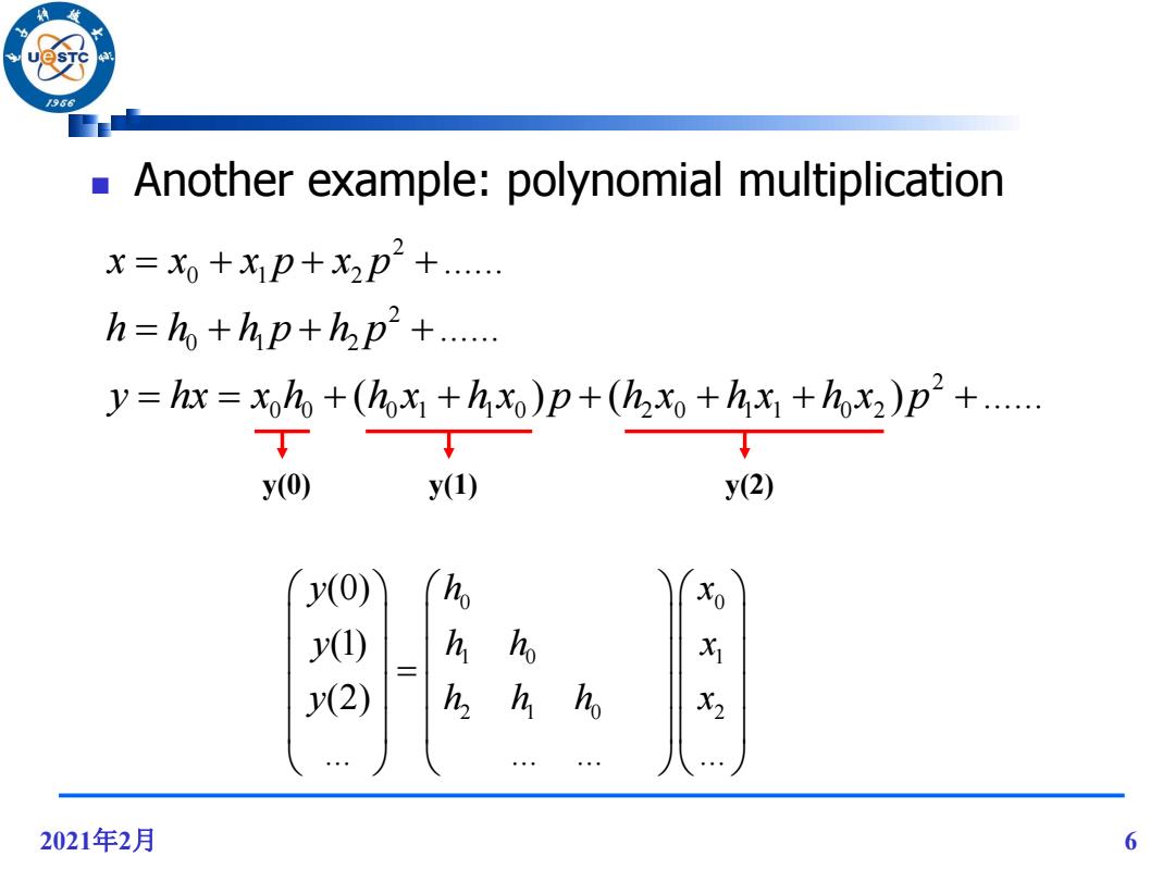
/96 Another example:polynomial multiplication X=x0+X1p+X2p2+. h=ho+hp+hp+..... y=hx=xoho+(hohx)p+(h2x++hox2)p2+..... y(0) y(1) y(2) y(0) Xo y() h h 水 y(2) h h h X2 2021年2月 6
2021年2月 6 Another example: polynomial multiplication 2 0 1 2 2 0 1 2 2 0 0 0 1 1 0 2 0 1 1 0 2 ...... ...... ( ) ( ) ...... x x x p x p h h h p h p y hx x h h x h x p h x h x h x p y(0) y(1) y(2) 0 0 1 0 1 2 1 0 2 (0) (1) (2) ... ... ... ... y h x y h h x y h h h x
Fast convolution /96 In this chapter we will discuss two well-known approaches to the design of fast short-length convolution algorithms: ■ Cook-Toom algorithm (based on Lagrange Interpolation) Winograd Algorithm (based on the Chinese remainder theorem) 2021年2月 7
2021年2月 7 Fast convolution In this chapter we will discuss two well-known approaches to the design of fast short-length convolution algorithms: Cook-Toom algorithm (based on Lagrange Interpolation) Winograd Algorithm (based on the Chinese remainder theorem)
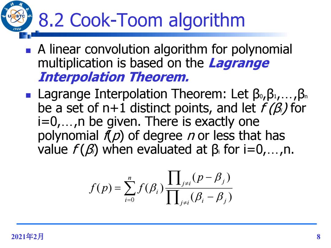
8.2 Cook-Toom algorithm /96 A linear convolution algorithm for polynomial multiplication is based on the Lagrange Interpolation Theorem. Lagrange Interpolation Theorem:Letβo,β:,..β be a set of n+1 distinct points,and let f()for i=0,...,n be given.There is exactly one polynomial p)of degree n or less that has value f(B)when evaluated at B for i=0,...,n. (p-B,) fp)=fBA,)T.B-B,) 2021年2月 8
2021年2月 8 8.2 Cook-Toom algorithm A linear convolution algorithm for polynomial multiplication is based on the Lagrange Interpolation Theorem. Lagrange Interpolation Theorem: Let β0,β1,…,βn be a set of n+1 distinct points, and let f (βi) for i=0,…,n be given. There is exactly one polynomial f(p) of degree n or less that has value f (βi) when evaluated at βi for i=0,…,n. n i j i i j j i j i p f p f 0 ( ) ( ) ( ) ( )

8.2 Cook-Toom algorithm 96 Polynomial multiplication s(p)=h(p)x(p) x(p)=x-1p-+●+xp+x0 h(p)=hw-1pN-+●●+hp+h degree s(p)=2+N-2D+N2++Sp+S0 L+N-1 coefficients If s(B),for i=0,1,...,L+N-2 are known,the unique s(p)can be computed as: L+N-2 s(p)=∑s(B,) Πp-B) i=0 Π(B,-B,) 9
9 8.2 Cook-Toom algorithm s( p) h( p)x( p) 1 0 1 1 h( p) h p h p h N N 1 1 1 0 ( ) L L x p x p x p x 2 2 1 0 ( ) L N L N s p s p s p s 2 0 ( ) ( ) ( ) ( ) L N i j i i j j i j i p s p s Polynomial multiplication If s(βi), for i=0,1,…,L+N-2 are known, the unique s(p) can be computed as: degree L+N-1 coefficients
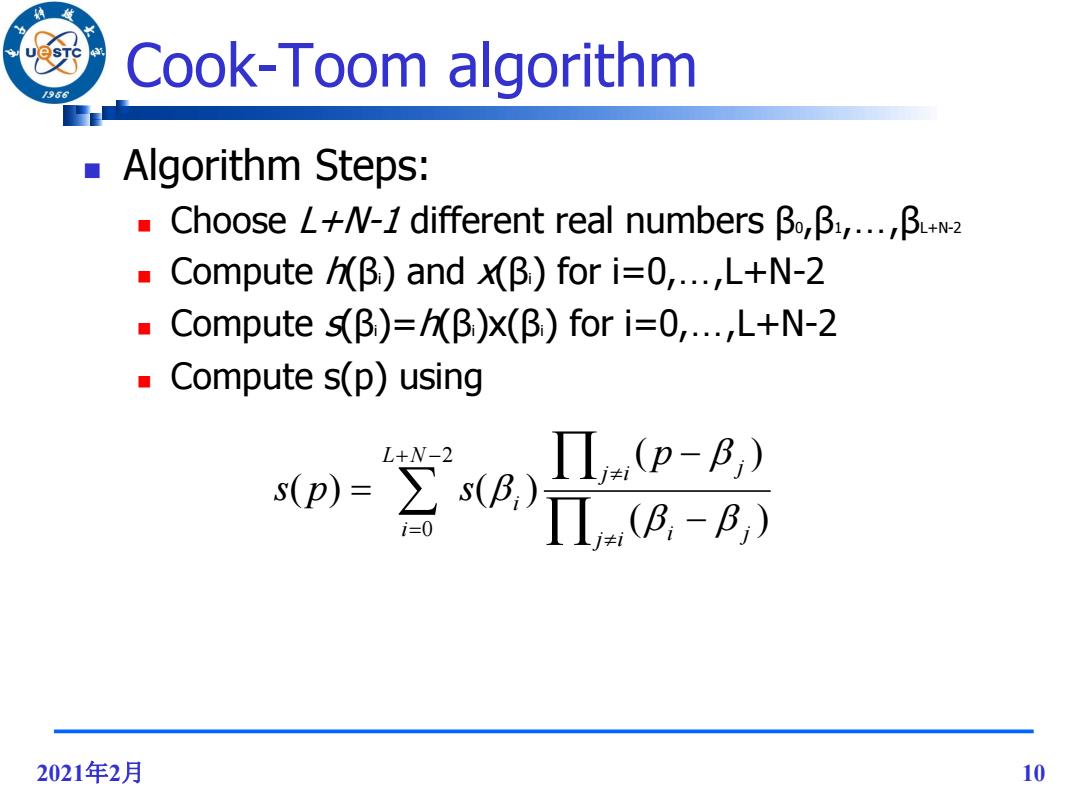
Cook-Toom algorithm 96 Algorithm Steps: ■Choose L+W-1 different real numbersβ,β,..,B+w2 Compute/B)and x(B)for i=0,...,L+N-2 ■Compute s(β)=hβ)x(β)fori=0,..,L+N-2 Compute s(p)using Π(p-B;) sp)=空g)7iB,-B L+N-2 i=0 2021年2月 10
2021年2月 10 Cook-Toom algorithm Algorithm Steps: Choose L+N-1 different real numbers β0,β1,…,βL+N-2 Compute h(βi) and x(βi) for i=0,…,L+N-2 Compute s(βi)=h(βi)x(βi) for i=0,…,L+N-2 Compute s(p) using 2 0 ( ) ( ) ( ) ( ) L N i j i i j j i j i p s p s