
Advanced Algorithms Greedy and Local Search 尹一通Nanjing University,2022Fall
尹⼀通 Nanjing University, 2022 Fall Advanced Algorithms Greedy and Local Search
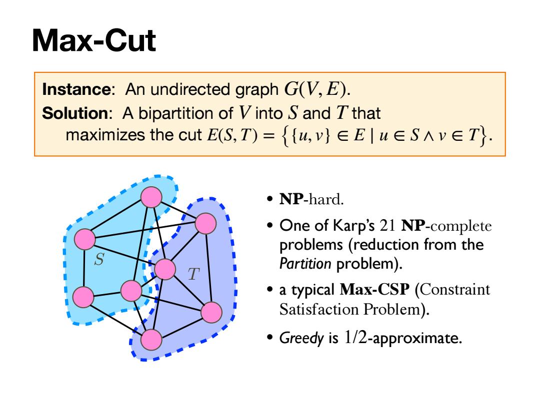
Max-Cut Instance:An undirected graph G(V,E). Solution:A bipartition of V into S and Ithat maximizes the cut E(S,T)={w,v}∈E|u∈S∧v∈T} .NP-hard. One of Karp's 21 NP-complete problems(reduction from the Partition problem). .a typical Max-CSP (Constraint Satisfaction Problem). Greedy is 1/2-approximate
Max-Cut Instance: An undirected graph . Solution: A bipartition of into and that maximizes the cut . G(V, E) V S T E(S, T) = {{u, v} ∈ E ∣ u ∈ S ∧ v ∈ T} T S • NP-hard. • One of Karp’s 21 NP-complete problems (reduction from the Partition problem). • a typical Max-CSP (Constraint Satisfaction Problem). • Greedy is 1/2-approximate
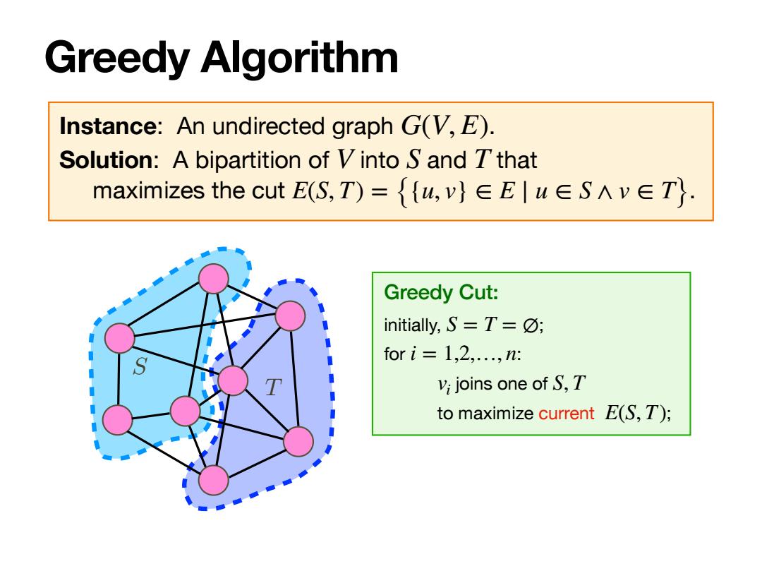
Greedy Algorithm Instance:An undirected graph G(V,E). Solution:A bipartition of Vinto S and Tthat maximizes the cut E(S,T)={w,v}∈E|w∈S∧v∈T}. Greedy Cut: initially,S=T=O; fori=1,2,.,n: Vi joins one of S,T to maximize current E(S,T);
Greedy Algorithm Instance: An undirected graph . Solution: A bipartition of into and that maximizes the cut . G(V, E) V S T E(S, T) = {{u, v} ∈ E ∣ u ∈ S ∧ v ∈ T} T S Greedy Cut: initially, ; for : joins one of to maximize current ; S = T = ∅ i = 1,2,…, n vi S, T E(S, T)
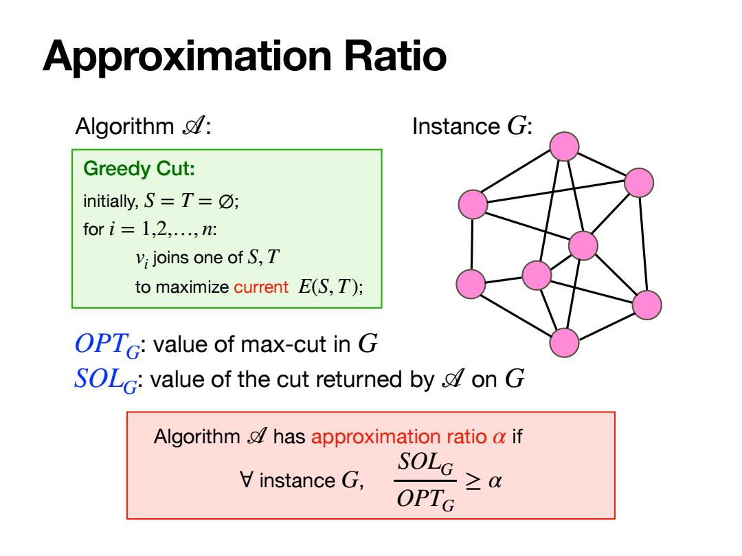
Approximation Ratio Algorithm & Instance G: Greedy Cut: initially,S=T=O; fori=1,2,.,n: Vi joins one of S,T to maximize current E(S,T); OPTG:value of max-cut in G SOLG:value of the cut returned by on G Algorithm has approximation ratio a if SOLG V instance G, ≥ OPTG
Approximation Ratio Greedy Cut: initially, ; for : joins one of to maximize current ; S = T = ∅ i = 1,2,…, n vi S, T E(S, T) Algorithm 𝒜: Instance G: : value of max-cut in : value of the cut returned by on OPTG G SOLG 𝒜 G Algorithm has approximation ratio if instance , 𝒜 α ∀ G SOLG OPTG ≥ α
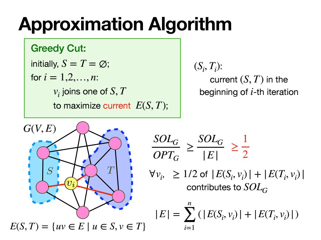
Approximation Algorithm Greedy Cut: initially,S=T=; (S,T: fori=1,2,.,n: current (S,T)in the Vi joins one of S,T beginning of i-th iteration to maximize current E(S,T); G(V,E) SOLG SOLG 1 OPTG ≥ |E1 v≥1/2of|E(S,)川+|E(T)l contributes to SOLG IEI=∑(IES,l+IET,I) E(S,T)={uv∈E|u∈S,v∈T} i=1
Approximation Algorithm E(S, T) = {uv ∈ E ∣ u ∈ S, v ∈ T} Greedy Cut: initially, ; for : joins one of to maximize current ; S = T = ∅ i = 1,2,…, n vi S, T E(S, T) S T vi G(V, E) SOLG OPTG ≥ SOLG |E| , of contributes to ∀vi ≥ 1/2 |E(Si , vi )| + |E(Ti , vi )| SOLG ≥ 1 2 |E| = n ∑ i=1 (|E(Si , vi )| + |E(Ti , vi )|) : current in the beginning of -th iteration (Si , Ti ) (S, T) i
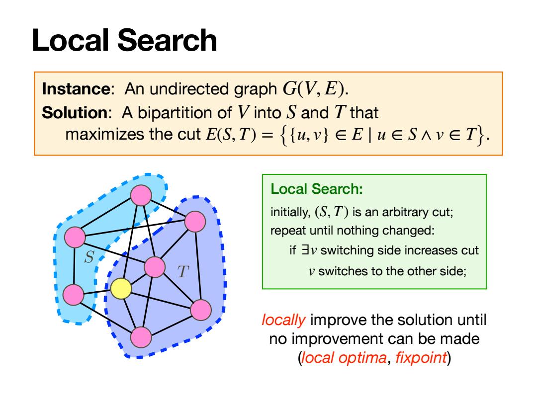
Local Search Instance:An undirected graph G(V,E). Solution:A bipartition of V into S and T that maximizes the cut E(S,T)={w,v}∈Eluw∈S∧v∈T}. Local Search: initially,(S,T)is an arbitrary cut; repeat until nothing changed: if v switching side increases cut v switches to the other side; locally improve the solution until no improvement can be made (local optima,fixpoint)
Local Search Instance: An undirected graph . Solution: A bipartition of into and that maximizes the cut . G(V, E) V S T E(S, T) = {{u, v} ∈ E ∣ u ∈ S ∧ v ∈ T} Local Search: initially, is an arbitrary cut; repeat until nothing changed: if switching side increases cut switches to the other side; (S, T) ∃v v locally improve the solution until no improvement can be made (local optima, fixpoint) T S

Local Search Local Search: initially,(S,T)is an arbitrary cut; repeat until nothing changed: ifv switching side increases cut v switches to the other side; in a local optima: v∈S:|E(y,S)川≤|E(y,T)川→21E(S,S)川≤|E(S,T)川 v∈T:|E(y,T)川≤IE(y,S)l→2|E(T,T)川≤IE(S,T)l E(S,S)+E(T,T)<E(S,T) OPT≤IE1=IE(S,S)川+IE(T,T)川+IE(S,T)I≤2|E(S,T)I →IE(S,T)I≥二OPT
Local Search Local Search: initially, is an arbitrary cut; repeat until nothing changed: if switching side increases cut switches to the other side; (S, T) ∃v v in a local optima: ∀v ∈ S : |E(v, S)| ≤ |E(v, T)| ⟹ 2|E(S, S)| ≤ |E(S, T)| ∀v ∈ T : |E(v, T)| ≤ |E(v, S)| ⟹ 2|E(T, T)| ≤ |E(S, T)| |E(S, S)| + |E(T, T)| ≤ |E(S, T)| OPT ≤ |E| = |E(S, S)| + |E(T, T)| + |E(S, T)| ⟹ |E(S, T)| ≥ 1 2 OPT ≤ 2|E(S, T)| T S

Scheduling
Scheduling
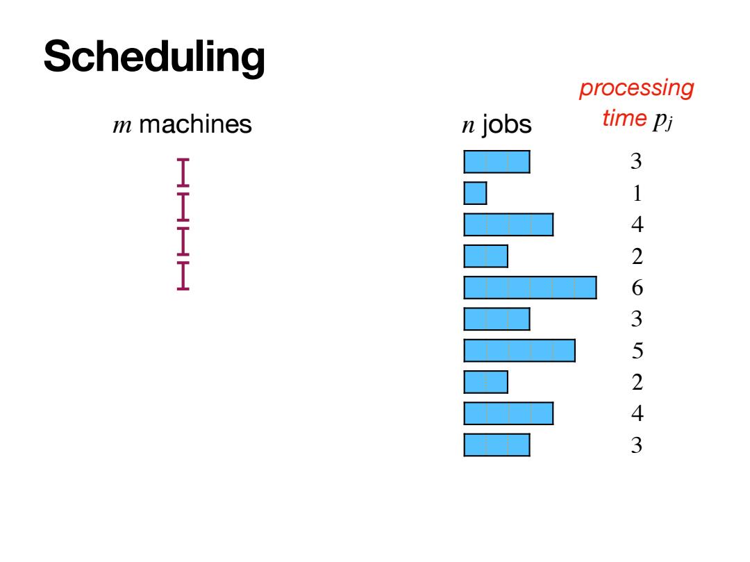
Scheduling processing m machines n jobs time pj 3 HH 9 1 4 HH 2 6 3 5 2 4 3
Scheduling m machines n jobs processing time pj 3 1 4 2 6 3 5 2 4 3
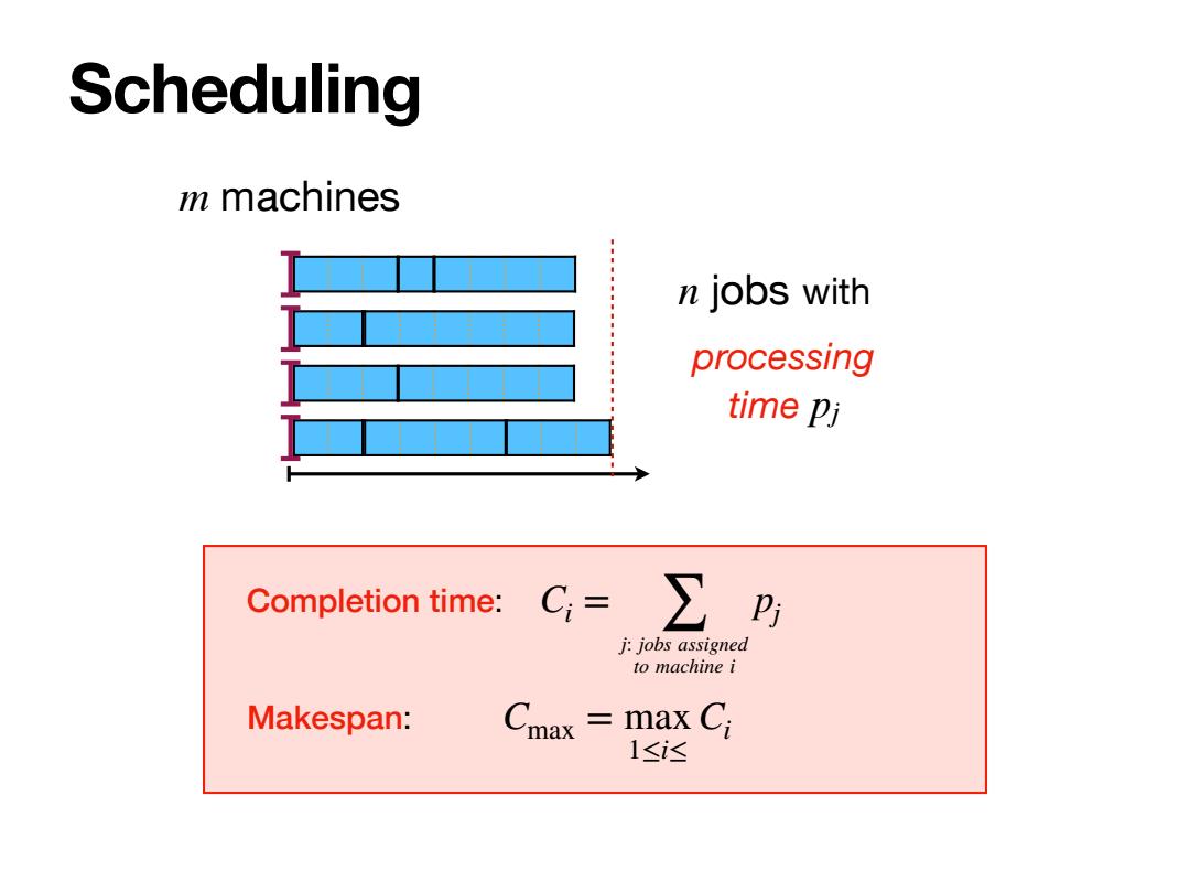
Scheduling m machines n jobs with processing time Pj Completion time: C=∑ j:jobs assigned to machine i Makespan: max ma <Ci 1≤i达
Scheduling n jobs m machines processing time pj with Completion time: Makespan: Ci = j: job ∑ s assigned to machine i pj Cmax = max 1≤i≤ Ci