
Computer Simulation of liquids M.P.ALLEN H.H.Wills Physics Laboratory University of Bristol and D.J.TILDESLEY Department of Chemistry The University,Southampton CLARENDON PRESS OXFORD
To Diane and Pauline
PREFACE This is a 'how-to-do-it'book for people who want to use computers to simulate the behaviour of atomic and molecular liquids.We hope that it will be useful to first-year graduate students,research workers in industry and academia,and to teachers and lecturers who want to use the computer to illustrate the way liquids behave. Getting started is the main barrier to writing a simulation program.Few people begin their research into liquids by sitting down and composing a program from scratch.Yet these programs are not inherently complicated: there are just a few pitfalls to be avoided.In the past,many simulation programs have been handed down from one research group to another and from one generation of students to the next.Indeed,with a trained eye,it is possible to trace many programs back to one of the handful of groups working in the field 20 years ago.Technical details such as methods for improving the speed of the program or for avoiding common mistakes are often buried in the appendices of publications or passed on by word of mouth.In the first six chapters of this book,we have tried to gather together these details and to present a clear account of the techniques,namely Monte Carlo and molecular dynamics.The hope is that a graduate student could use these chapters to write his own program. The field of computer simulation has enjoyed rapid advances in the last five years.Smart Monte Carlo sampling techniques have been introduced and tested,and the molecular dynamics method has been extended to simulate various ensembles.The techniques have been merged into a new field of stochastic simulations and extended to cover quantum-mechanical as well as classical systems.A book on simulation would be incomplete without some mention of these advances and we have tackled them in Chapters 7 to 10. Chapter 1I contains a brief account of some interesting problems to which the methods have been applied.Our choices in this chapter are subjective and our coverage far from exhaustive.The aim is to give the reader a taste rather than a feast.Finally we have included examples of computer code to illustrate points made in the text,and have provided a wide selection of useful routines which are available on-line from two sources.We have not attempted to tackle the important areas of solid state simulation and protein molecular mechanics. The techniques discussed in this book are useful in these fields,but additionally much weight is given to energy minimization rather than the simulation of systems at non-zero temperatures.The vast field of lattice dynamics is discussed in many other texts. Both of us were fortunate in that we had expert guidance when starting work in the field,and we would like to take this opportunity to thank P.Schofield (Harwell)and W.B.Streett (Cornell),who set us on the right

viii PREFACE road some years ago.This book was largely written and created at the Physical Chemistry Laboratory,Oxford,where both of us have spent a large part of our research careers.We owe a great debt of gratitude to the head of department,J.S.Rowlinson,who has provided us with continuous en- couragement and support in this venture,as well as a meticulous criticism of early versions of the manuscript.We would also like to thank our friends and colleagues in the Physics department at Bristol and the Chemistry depart- ment at Southampton for their help and encouragement,and we are indebted to many colleagues,who in discussions at conferences and workshops, particularly those organized by CCP5 and CECAM,have helped to form our ideas.We cannot mention all by name,but should say that conversations with D.Frenkel and P.A.Madden have been especially helpful.We would also like to thank M.Gillan and J.P.Ryckaert,who made useful comments on certain chapters,and I.R.McDonald who read and commented on the completed manuscript.We are grateful for the assistance of Mrs L.Hayes,at Oxford University Computing Service,where the original Microfiche was produced. Lastly,we thank Taylor and Francis for allowing us to reproduce diagrams from Molecular Physics and Advances in Physics,and ICL and Cray Research (UK)for the photographs in Fig.1.1.Detailed acknowledgements appear in the text. Books are not written without a lot of family support.One of us(DJT) wants to thank the Oaks and the Sibleys of Bicester for their hospitality during many weekends in the last three years.Our wives,Diane and Pauline,have suffered in silence during our frequent disappearances,and given us their unflagging support during the whole project.We owe them a great deal. Bristol M.P.A. Southampton D.J.T. May 1986

CONTENTS LIST OF SYMBOLS I INTRODUCTION 1 1.1 A short history of computer simulation 1 1.2 Computer simulation:motivation and applications 4 1.3 Model systems and interaction potentials 6 1.3.1 Introduction 6 1.3.2 Atomic systems 7 1.3.3 Molecular systems 12 1.3.4 Lattice systems 16 1.3.5 Calculating the potential 18 1.4 Constructing an intermolecular potential 1.4.1 Introduction 1.4.2 Building the model potential 1.4.3 Adjusting the model potential 1.5 Studying small systems 1.5.1 Introduction 1.5.2 Periodic boundary conditions 1.5.3 Potential truncation 20000023234792 1.5.4 Computer code for periodic boundaries 1.5.5 Spherical boundary conditions 2 STATISTICAL MECHANICS 33 2.1 Sampling from ensembles 2.2 Common statistical ensembles 3339 2.3 Transforming between ensembles 43 2.4 Simple thermodynamic averages 46 2.5 Fluctuations 51 2.6 Structural quantities 54 2.7 Time correlation functions and transport coefficients 58 2.8 Long-range corrections 64 2.9 Quantum corrections 65 2.10 Constraints 68 3 MOLECULAR DYNAMICS 71 3.1 Equations of motion for atomic systems 71 3.2 Finite difference methods 3 3.2.1 The Verlet algorithm 78 3.2.2 The Gear predictor-corrector 8 3.2.3 Other methods 84 3.3 Molecular dynamics of rigid non-spherical bodies 3.3.I Non-linear molecules 8 3.3.2 Linear molecules 90
CONTENTS 3.4 Constraint dynamics 92 3.5 Checks on accuracy 3.6 Molecular dynamics of hard systems 101 3.6.1 Hard spheres 102 3.6.2 Hard non-spherical bodies 108 4 MONTE CARLO METHODS 110 4.1 Introduction 110 4.2 Monte Carlo integration 111 4.2.1 Hit and miss 111 4.2.2 Sample mean integration 112 4.3 Importance sampling 114 4.4 The Metropolis method 118 4.5 Isothermal-isobaric Monte Carlo 123 4.6 Grand canonical Monte Carlo 126 4.7 Molecular liquids 131 4.7.1 Rigid molecules 131 4.7.2 Non-rigid molecules 135 5 SOME TRICKS OF THE TRADE 140 5.1 Introduction 140 5.2 The heart of the matter 140 5.2.1 Efficient calculation of forces,energies,and pressures 140 5.2.2 Avoiding the square root 143 5.2.3 Table look-up and spline-fit potentials 143 5.2.4 Shifted and shifted-force potentials 145 5.3 Neighbour lists 146 5.3.1 The Verlet neighbour list 147 5.3.2 Cell structures and linked lists 149 5.4 Multiple time step methods 152 5.5 How to handle long-range forces 155 5.5.1 Introduction 155 5.5.2 The Ewald sum 156 5.5.3 The reaction field method 162 5.5.4 Other methods 164 5.5.5 Summary 164 5.6 When the dust has settled 166 5.7 Starting up 168 5.7.1 The initial configuration 168 5.7.2 The initial velocities 170 5.7.3 Equilibration 171 5.8 Organization of the simulation 173 5.8.1 Input/output and file handling 174 5.8.2 Program structure 175 5.8.3 The scheme in action 180 6 HOW TO ANALYSE THE RESULTS 182 6.1 Introduction 182 6.2 Liquid structure 183
CONTENTS xi 6.3 Time correlation functions 185 6.3.1 The direct approach 185 6.3.2 The fast Fourier transform method 188 6.4 Estimating errors 191 6.4.I Errors in equilibrium averages 192 6.4.2 Errors in fluctuations 195 6.4.3 Errors in structural quantities 195 6.4.4 Errors in time correlation functions 196 6.5 Correcting the results 198 6.5.1 Correcting thermodynamic averages 199 6.5.2 Extending g(r)to large r 199 6.5.3 Extrapolating g(r)to contact 201 6.5.4 Smoothing g(r) 203 6.5.5 Calculating transport coefficients 204 6.5.6 Smoothing a spectrum 208 7 ADVANCED SIMULATION TECHNIQUES 212 7.1 Introduction 212 7.2 Free energy estimation 213 7.2.1 Introduction 213 7.2.2 Non-Boltzmann sampling 213 7.2.3 Acceptance ratio method 218 7.2.4 Summary 219 7.3 Smarter Monte Carlo 220 7.3.I Preferential sampling 220 7.3.2 Force-bias Monte Carlo 224 7.3.3 Smart Monte Carlo 225 7.3.4 Virial-bias Monte Carlo 226 7.4 Constant-temperature molecular dynamics 227 7.4.1 Stochastic methods 227 7.4.2 Extended system methods 228 7.4.3 Constraint methods 230 7.4.4 Other methods 23】 7.5 Constant-pressure molecular dynamics 232 7.5.1 Extended system methods 232 7.5.2 Constraint methods 234 7.5.3 Other methods 236 7.5.4 Changing box shape 236 7.6 Practical points 238 7.7 The Gibbs Monte Carlo method 239 8 NON-EQUILIBRIUM MOLECULAR DYNAMICS 240 8.1 Introduction 240 8.2 Shear flow 242 8.3 Expansion and contraction 249 8.4 Heat flow 250 8.5 DifTusion 251 8.6 Other perturbations 253 8.7 Practical points 253
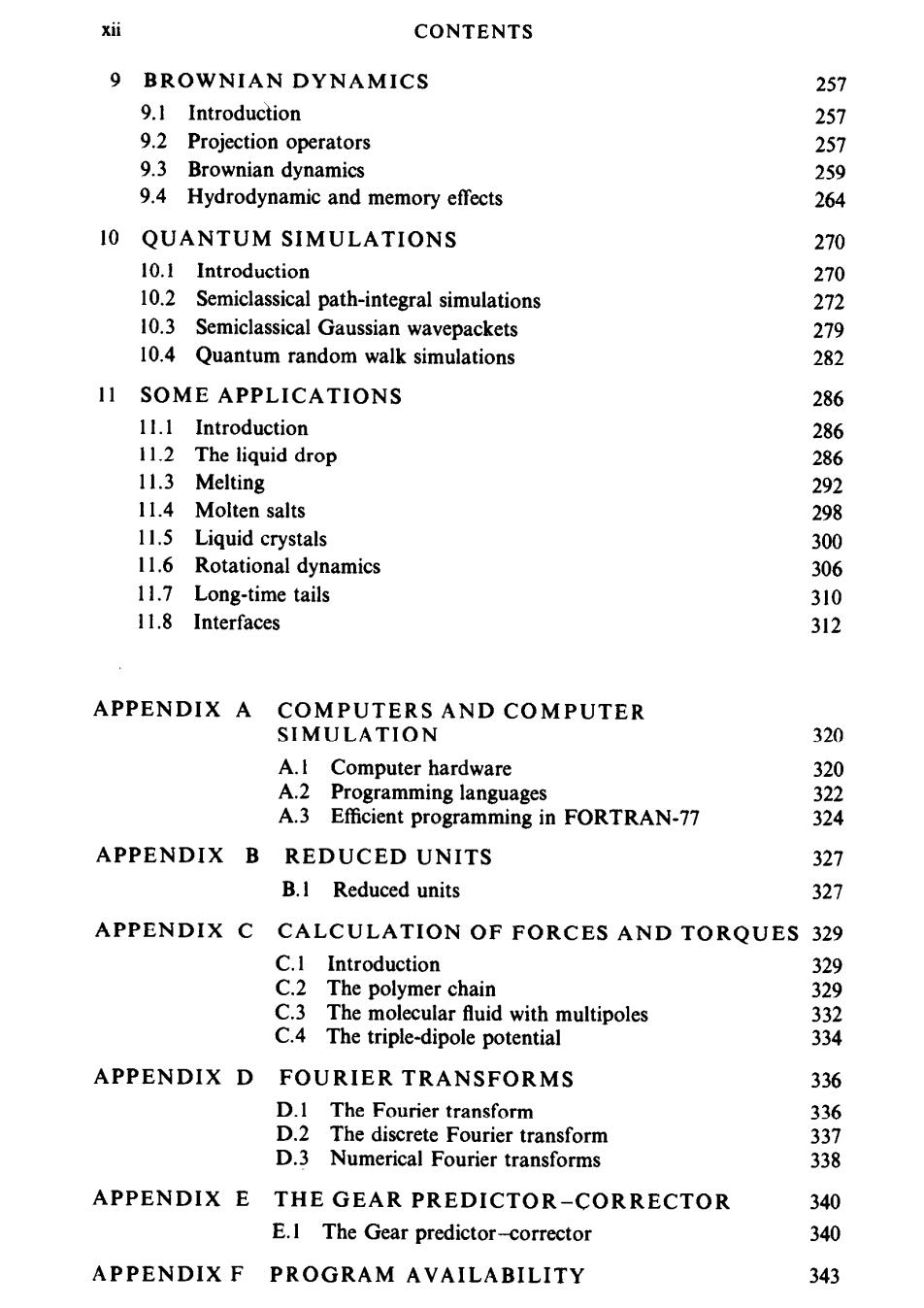
xii CONTENTS 9 BROWNIAN DYNAMICS 257 9.1 Introduction 257 9.2 Projection operators 257 9.3 Brownian dynamics 259 9.4 Hydrodynamic and memory effects 264 10 QUANTUM SIMULATIONS 270 10.1 Introduction 270 10.2 Semiclassical path-integral simulations 272 10.3 Semiclassical Gaussian wavepackets 279 10.4 Quantum random walk simulations 282 11 SOME APPLICATIONS 286 11.1 Introduction 286 11.2 The liquid drop 286 11.3 Melting 292 11.4 Molten salts 298 11.5 Liquid crystals 300 11.6 Rotational dynamics 306 11.7 Long-time tails 310 11.8 Interfaces 312 APPENDIX A COMPUTERS AND COMPUTER SIMULATION 320 A.I Computer hardware 320 A.2 Programming languages 322 A.3 Efficient programming in FORTRAN-77 324 APPENDIX B REDUCED UNITS 327 B.1 Reduced units 327 APPENDIX C CALCULATION OF FORCES AND TORQUES 329 C.1 Introduction 329 C.2 The polymer chain 329 C.3 The molecular fluid with multipoles 332 C.4 The triple-dipole potential 334 APPENDIX D FOURIER TRANSFORMS 336 D.1 The Fourier transform 336 D.2 The discrete Fourier transform 337 D.3 Numerical Fourier transforms 338 APPENDIX E THE GEAR PREDICTOR-CORRECTOR 340 E.I The Gear predictor-corrector 340 APPENDIX F PROGRAM AVAILABILITY 343

CONTENTS xi近 APPENDIX G RANDOM NUMBERS 345 G.1 Random number generators 345 G.2 Random numbers uniform on(0,1) 345 G.3 Generating non-uniform distributions 347 G.4 Random vectors on the surface of a sphere 349 G.5 Choosing randomly and uniformly from complicated regions 349 G.6 Sampling from an arbitrary distribution 351 REFERENCES 352 INDEX 383
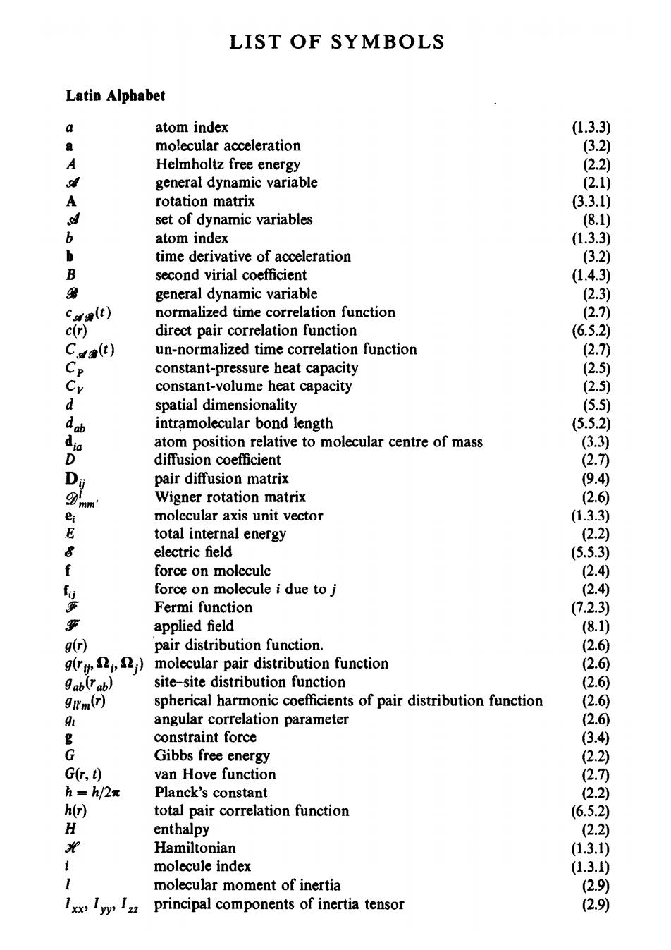
LIST OF SYMBOLS Latin Alphabet a atom index (1.3.3) ” molecular acceleration (3.2) A Helmholtz free energy (2.2) Q7 general dynamic variable (2.1) A rotation matrix 3.3.1) 4 set of dynamic variables (8.1) 6 atom index (1.3.3) b time derivative of acceleration (3.2) B second virial coefficient (1.4.3) 第 general dynamic variable (2.3) cw(t) normalized time correlation function (2.7) c(r) direct pair correlation function (6.5.2) Cda(t) un-normalized time correlation function (2.7) CP constant-pressure heat capacity (2.5 constant-volume heat capacity (2.5) spatial dimensionality (5.5) dab intramolecular bond length (5.5.2) atom position relative to molecular centre of mass (3.3) D diffusion coefficient (2.7) D可 pair diffusion matrix (9.4) 9hm' Wigner rotation matrix (2.6) molecular axis unit vector (1.3.3) E total internal energy (2.2) 8 electric field (5.5.3) force on molecule (2.4) f force on molecule i due to j (2.4) Fermi function (7.2.3) 等 applied field (8.1) g(r) pair distribution function. (2.6) g(ry DiR;) molecular pair distribution function (2.6) gab(rab) site-site distribution function (2.6) 9Im(r) spherical harmonic coefficients of pair distribution function (2.6) 91 angular correlation parameter (2.6) g constraint force 3.4) G Gibbs free energy (2.2) G(r,t) van Hove function 2.7) h=h/2π Planck's constant (2.2) h(r) total pair correlation function (6.5.2) H enthalpy (2.2) 3光 Hamiltonian (1.3.1) molecule index (1.3.1) 1 molecular moment of inertia (2.9) principal components of inertia tensor (2.9)